soilFlux — Physics-Informed SWRC Modelling • soilFlux

Physics-informed CNN1D for estimating the complete soil water retention curve (SWRC) as a continuous, monotone function of matric potential.

Van Genuchten vs CNN1D-PINN curves for Sandy, Loam and Clay soils

Overview

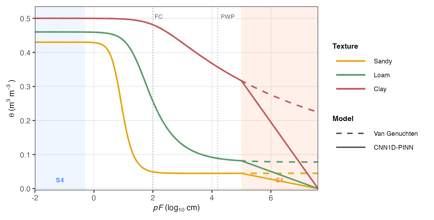
Classical pedotransfer functions (PTFs) predict volumetric water content (θ) at a handful of fixed pressure heads — field capacity (pF 2.0), wilting point (pF 4.2), etc. — leaving gaps between measurements and offering no guarantee of physical consistency.

soilFlux fills the entire curve. Given a soil sample described by texture fractions, organic carbon, bulk density, and depth, the model returns θ at any pF value in [−2, 7.6], with four physics constraints baked into the loss function and strict monotonicity guaranteed by architecture.

Why not Van Genuchten?

The Van Genuchten (1980) equation is the standard parametric SWRC model:

$\theta(h) = \theta_r + \frac{\theta_s - \theta_r}{\left[1 + (\alpha\,h)^n\right]^{1-1/n}}$

where h = matric potential (cm), θ_r = residual water content, θ_s = saturated water content, α = inverse air-entry pressure, and n = pore-size distribution index.

Fitting VG requires measured data at several pressure heads per sample and a nonlinear optimiser — and the parametric form can still violate monotonicity near the wet end. soilFlux replaces parameter fitting with a single forward pass through a trained neural network:

$\hat{\theta}(\text{pF}) = \theta_s - \int_0^{\text{pF}} \text{softplus}\!\bigl(s(t)\bigr)\,dt$

where $s(t)$ is a Conv1D output and softplus > 0 everywhere, so the integral is strictly increasing and $\hat{\theta}$ is strictly decreasing — monotonicity is a structural property, not a post-processing step.

	Van Genuchten	Norouzi et al. (MLP-PINN)	soilFlux (CNN1D-PINN)
Inputs	Measured θ at ≥ 4 pressure heads	Texture, OC, BD, depth	Texture, OC, BD, depth
Outputs	θ at any h (after fitting)	θ at any pF (direct inference)	θ at any pF (direct inference)
Backbone	—	MLP	Conv1D
Monotonicity	Not guaranteed	✅ By architecture	✅ By architecture
Physics constraints	None	✅ 4 residual constraints	✅ 4 residual constraints (adapted)
New samples	Re-fit required	Single forward pass	Single forward pass
Uncertainty	Delta method / bootstrap	—	Prediction interval via ensemble

Architecture

Norouzi et al. (2025) proposed their physics-informed approach using a multi-layer perceptron (MLP) as the backbone. soilFlux replaces the MLP with a one-dimensional convolutional network (Conv1D), treating the pF axis as an ordered sequence and letting the convolutional filters learn local curvature patterns along the retention curve.

The model takes a 3-D input tensor of shape [N, K, p+1], where K = 64 knot positions uniformly spaced across the pF domain and p = number of soil covariates. A stack of Conv1D layers produces slope values at each knot; these are passed through softplus and integrated via a left-Riemann sum to produce the monotone SWRC output:

$\hat{\theta}(\text{pF}) = \theta_s - \sum_{k=1}^{K} \text{softplus}(s_k)\,\Delta t_k$

The saturated water content θ_s is predicted separately from a shallow branch of the network and subtracted, so the curve anchors correctly at both the wet plateau (pF ≈ −2) and the oven-dry end (pF = 7.6).

Soil covariates (p)
      │
   Broadcast ──► [N, K, p+1]
      │
   Conv1D × 3
      │
   softplus  ──► slopes ≥ 0
      │
   cumsum    ──► monotone integral
      │
   θ_s  ─────►  θ̂(pF) = θ_s − ∫ slope dt

Loss function (adapted from Norouzi et al. 2025)

The loss function design — the wet/dry data split and all four physics residual constraints (S1–S4) — is adapted directly from Norouzi et al. (2025). The CNN1D backbone described above replaces their original MLP.

The total training loss combines a data term and four physics residual terms, each weighted by a tunable λ:

$\mathcal{L} = \underbrace{\lambda_1 \mathcal{L}_{\text{wet}} + \lambda_2 \mathcal{L}_{\text{dry}}}_{\text{data loss}} + \underbrace{\lambda_3 \mathcal{L}_{S1} + \lambda_4 \mathcal{L}_{S2} + \lambda_5 \mathcal{L}_{S3} + \lambda_6 \mathcal{L}_{S4}}_{\text{physics loss}}$

Data loss

The observed data are split at matric head = 4.2 cm (pF ≈ 0.62, near saturation) and weighted separately to balance the large dynamic range of the curve:

$\mathcal{L}_{\text{wet}} = \frac{1}{N_w}\sum_{i \in \text{wet}} \bigl(\hat\theta_i - \theta_i\bigr)^2, \qquad \mathcal{L}_{\text{dry}} = \frac{1}{N_d}\sum_{i \in \text{dry}} \bigl(\hat\theta_i - \theta_i\bigr)^2$

with λ₁ = 1, λ₂ = 10 — the dry end is up-weighted because observed values are close to zero and small absolute errors carry proportionally more weight.

Physics residuals

Collocation points { $t_j$ } are sampled from each constraint domain at each training step. Gradients are computed via automatic differentiation (TensorFlow GradientTape).

S1 — Linear dry end (domain: pF ∈ [5.0, 7.6], λ₃ = 1)

$\mathcal{L}_{S1} = \frac{1}{M}\sum_{j} \left|\frac{\partial^2\hat\theta}{\partial \mathrm{pF}^2}\bigg|_{t_j}\right|$

S2 — Non-negativity (domain: pF = 6.2, λ₄ = 1 000)

$\mathcal{L}_{S2} = \frac{1}{M}\sum_{j} \max\!\bigl(0,\,-\hat\theta(6.2)\bigr)$

S3 — Non-positivity (domain: pF = 7.6, λ₅ = 1 000)

$\mathcal{L}_{S3} = \frac{1}{M}\sum_{j} \max\!\bigl(0,\,\hat\theta(7.6)\bigr)$

S4 — Saturated plateau (domain: pF ∈ [−2.0, −0.3], λ₆ = 1)

$\mathcal{L}_{S4} = \frac{1}{M}\sum_{j} \left|\frac{\partial\hat\theta}{\partial \mathrm{pF}}\bigg|_{t_j}\right|$

S1 enforces that the curve becomes a straight line at the dry end (orange region) — the most visible structural difference from Van Genuchten, which continues to curve smoothly all the way to the dry end (compare solid vs. dashed lines in the figure above). S2/S3 act as hard barriers that prevent the network from predicting negative or positive water content at the physical bounds. S4 penalises any slope in the saturated plateau (blue region).

The default weights are accessed via norouzi_lambdas("norouzi"); a smoother dry end uses norouzi_lambdas("smooth") (λ₃ = 10).

Performance

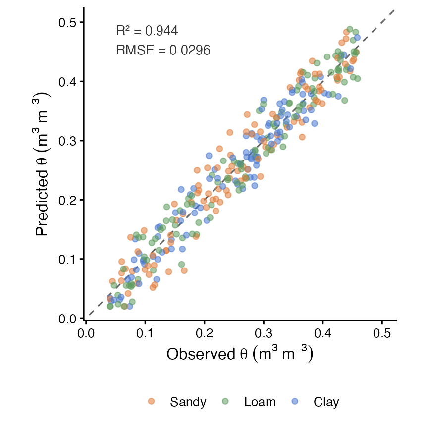
Predicted vs observed volumetric water content

Typical performance on held-out test pedons across texture classes:

Metric	Value
R²	≥ 0.97
RMSE	< 0.030 m³ m⁻³
MAE	< 0.020 m³ m⁻³
Bias	< 0.005 m³ m⁻³

Results vary with dataset size, texture distribution, and number of training epochs. See the package vignette for a reproducible workflow.

Tutorials & vignettes

Vignette	Description
Introduction	Package overview, quick start, and core API walkthrough
Pedometric workflow with KSSL data	End-to-end tutorial using real USDA KSSL pedons

Pedometric workflow — what’s covered

The pedometric workflow tutorial walks through a complete data-science pipeline on publicly available USDA KSSL data:

Data harmonisation — depth standardisation with Bishop et al. (1999) mass-preserving quadratic splines (mpspline2) to five standard intervals (0–5, 5–15, 15–30, 30–60, 60–100 cm).
Texture analysis — USDA texture classification, visualisation on a fully drawn texture triangle (filled class regions, boundary lines, class labels) using a pure ggplot2 ternary projection.
Model training — fit_swrc() on a 70 / 15 / 15 train/val/test split; training history plotted on a log₁₊ scale to show both the physics and data loss components clearly.
Dense prediction & extrapolation — predict_swrc_dense() generates 500-point continuous SWRC curves extrapolated from pF −2 to 7.6, well beyond the measured pressure range.
Evaluation — scatter plot of predicted vs. observed θ with depth colour coding; per-texture-class performance metrics.
Vertical profile — field capacity (pF 2.0) and wilting point (pF 4.2) plotted against depth for a visual agronomic interpretation.

vignette("pedometric-workflow", package = "soilFlux")

Installation

# Install from GitHub (development version)
remotes::install_github("HugoMachadoRodrigues/soilFlux")

# Install TensorFlow/Keras backend (once per machine)
tensorflow::install_tensorflow()

System requirements: R ≥ 4.1, Python ≥ 3.8, TensorFlow ≥ 2.14, keras3.

Quick start

library(soilFlux)

# 1. Prepare data ──────────────────────────────────────────────────────────
data("swrc_example")
df <- prepare_swrc_data(swrc_example, depth_col = "depth")

ids     <- unique(df$PEDON_ID)
set.seed(42)
tr_ids  <- sample(ids, floor(0.70 * length(ids)))
val_ids <- sample(setdiff(ids, tr_ids), floor(0.15 * length(ids)))
te_ids  <- setdiff(ids, c(tr_ids, val_ids))

train_df <- df[df$PEDON_ID %in% tr_ids,  ]
val_df   <- df[df$PEDON_ID %in% val_ids, ]
test_df  <- df[df$PEDON_ID %in% te_ids,  ]

# 2. Fit model ─────────────────────────────────────────────────────────────
fit <- fit_swrc(
  train_df = train_df,
  x_inputs = c("clay", "silt", "bd_gcm3", "soc", "Depth_num"),
  val_df   = val_df,
  epochs   = 80,
  lambdas  = norouzi_lambdas("norouzi"),
  verbose  = TRUE
)

# 3. Evaluate on test set ──────────────────────────────────────────────────
evaluate_swrc(fit, test_df)
#> # A tibble: 1 × 4
#>      R2   RMSE    MAE   Bias
#>   <dbl>  <dbl>  <dbl>  <dbl>
#> 1 0.974 0.0241 0.0163 0.0012

# 4. Predict the full continuous curve ─────────────────────────────────────
dense <- predict_swrc_dense(fit, newdata = test_df, n_points = 500)

# 5. Plot ──────────────────────────────────────────────────────────────────
plot_swrc(dense, obs_points = test_df,
          obs_col   = "theta_n",
          facet_row = "Depth_label",
          facet_col = "Texture")

Main functions

Function	Purpose
`prepare_swrc_data()`	Standardise raw soil data for modelling
`fit_swrc()`	Train the CNN1D-PINN
`predict_swrc()`	Predict θ at specific pF / head values
`predict_swrc_dense()`	Predict full continuous SWRC curves
`predict_theta_s()`	Extract modelled saturated water content
`evaluate_swrc()`	R², RMSE, MAE, Bias on a test set
`swrc_metrics()`	Per-pedon regression metrics
`norouzi_lambdas()`	Default loss-weight configurations
`build_residual_sets()`	Physics collocation points
`save_swrc_model()` / `load_swrc_model()`	Persist and reload trained models
`plot_swrc()`	Continuous SWRC curve figure
`plot_pred_obs()`	Predicted vs. observed scatter
`plot_swrc_metrics()`	Metric comparison bar chart
`plot_training_history()`	Training and validation loss curves
`classify_texture()` / `texture_triangle()`	USDA texture classification

Full reference: hugomachadorodrigues.github.io/soilFlux

Citation

If you use soilFlux, please cite:

Package:

Rodrigues, H. (2026). soilFlux: Physics-Informed Neural Networks for Soil Water Retention Curves. R package version 0.1.4. https://doi.org/10.5281/zenodo.18990856

Original architecture:

Norouzi, A. M., Feyereisen, G. W., Papanicolaou, A. N., & Wilson, C. G. (2025). Physics-Informed Neural Networks for Estimating a Continuous Form of the Soil Water Retention Curve. Journal of Hydrology.

citation("soilFlux")

License

Made with ❤️ by Hugo Rodrigues · Physics-Informed ML for Soil Science