Pedometric Workflow: KSSL Data, Spline Harmonisation, and SWRC Fitting

Backend note: Sections 1–6 (data download, splines, exploration) run without TensorFlow. Sections 7–9 (model fitting, prediction, evaluation) require a working TensorFlow/Keras installation — those chunks are marked eval = FALSE. Run ?soilFlux for setup instructions.

Why harmonise horizons?

Soil survey data is collected at natural genetic horizons whose boundaries reflect pedogenic processes — an Ap horizon might extend 0–22 cm in one profile and 0–8 cm in the next. Before fitting a spatially continuous model (or any regression) we need observations on a common support.

The GlobalSoilMap framework (Arrouays et al. 2014) and ISRIC SoilGrids both adopt five standard depth intervals:

Interval	Midpoint	Rationale
0–5 cm	2.5	Surface organic matter, tillage layer
5–15 cm	10.0	Shallow root zone, topsoil
15–30 cm	22.5	Subsoil transition
30–60 cm	45.0	Rooting depth limit for most crops
60–100 cm	80.0	Deep subsoil / parent material

The correct harmonisation method is the mass-preserving (equal-area) quadratic spline of Bishop et al. (1999), implemented in the mpspline2 package. This spline:

fits a piecewise quadratic through horizon mid-points,
exactly preserves the mean value of each original horizon (mass conservation),
provides a smooth, continuous depth function that can be evaluated at any depth or integrated over any interval.

Required packages

install.packages(c("soilDB", "aqp", "mpspline2", "ggridges", "dplyr",
                   "tidyr", "ggplot2", "purrr"))
# remotes::install_github("HugoMachadoRodrigues/soilFlux")

library(soilFlux)
library(dplyr)
library(tidyr)
library(ggplot2)
library(purrr)

The mass-preserving spline — illustrated

Before applying splines to real data, we look at how they behave using a single synthetic profile. This makes the mechanics transparent.

if (!requireNamespace("mpspline2", quietly = TRUE))
  stop("Install mpspline2: install.packages('mpspline2')")

library(mpspline2)

# ── Synthetic profile ────────────────────────────────────────────────────────
hz_demo <- data.frame(
  id   = rep("Profile A", 5),
  top  = c(  0, 10, 25, 55,  90),
  bot  = c( 10, 25, 55, 90, 130),
  clay = c( 10, 16, 30, 38,  40)   # % clay — typical Ultisol argillic increase
)

std_d <- c(0, 5, 15, 30, 60, 100)   # GlobalSoilMap standard depths

# ── Fit spline ───────────────────────────────────────────────────────────────
sp <- mpspline2::mpspline(
  obj      = hz_demo,
  var_name = "clay",
  d        = std_d,
  vlow     = 0,
  vhigh    = 100
)

# Continuous 1-cm curve (100 values, depths 0–99 cm)
sp_curve <- data.frame(
  depth_cm = seq(0, 99),
  clay     = sp[[1]]$est_1cm
)

# Circles plotted AT the spline curve value at each interval midpoint
# (depth 2.5→ index 3, 10→11, 22.5→23, 45→46, 80→81 in 1-indexed vector)
std_mids <- c(2.5, 10, 22.5, 45, 80)
sp_pts <- data.frame(
  depth_mid = std_mids,
  clay      = sp[[1]]$est_1cm[floor(std_mids) + 1L]
)

# ── Plot ─────────────────────────────────────────────────────────────────────
ggplot() +
  # Original horizon rectangles
  geom_rect(
    data = hz_demo,
    aes(xmin = 0, xmax = clay, ymin = top, ymax = bot),
    fill = "sienna3", alpha = 0.25, colour = "sienna4", linewidth = 0.4
  ) +
  # Horizon mean bars
  geom_segment(
    data = hz_demo %>% mutate(mid = (top + bot) / 2),
    aes(x = 0, xend = clay, y = mid, yend = mid),
    colour = "sienna4", linewidth = 1.2
  ) +
  geom_point(
    data = hz_demo %>% mutate(mid = (top + bot) / 2),
    aes(x = clay, y = mid),
    colour = "sienna4", size = 3, shape = 16
  ) +
  # Continuous spline (0–99 cm)
  geom_line(
    data = sp_curve,
    aes(x = clay, y = depth_cm),
    colour = "steelblue4", linewidth = 1
  ) +
  # Open circles ON the spline at GlobalSoilMap interval midpoints
  geom_point(
    data = sp_pts,
    aes(x = clay, y = depth_mid),
    shape = 21, fill = "white", colour = "steelblue4",
    size = 4, stroke = 1.8
  ) +
  # GlobalSoilMap depth boundaries
  geom_hline(
    yintercept = std_d[-1],
    linetype = "dashed", colour = "grey50", linewidth = 0.4
  ) +
  annotate("text", x = 34, y = std_d[-1] + 1.5,
           label = paste0(std_d[-1], " cm"),
           size = 3, colour = "grey40", hjust = 0) +
  scale_y_reverse(limits = c(100, 0), breaks = seq(0, 100, 10)) +
  scale_x_continuous(limits = c(0, 45), expand = c(0, 0.5)) +
  labs(
    title    = "Mass-preserving spline harmonisation",
    subtitle = "Brown = original horizon means  |  Blue curve = spline  |  Open circles = spline at standard-depth midpoints",
    x = "Clay (%)",
    y = "Depth (cm)"
  ) +
  theme_minimal(base_size = 13) +
  theme(panel.grid.minor = element_blank())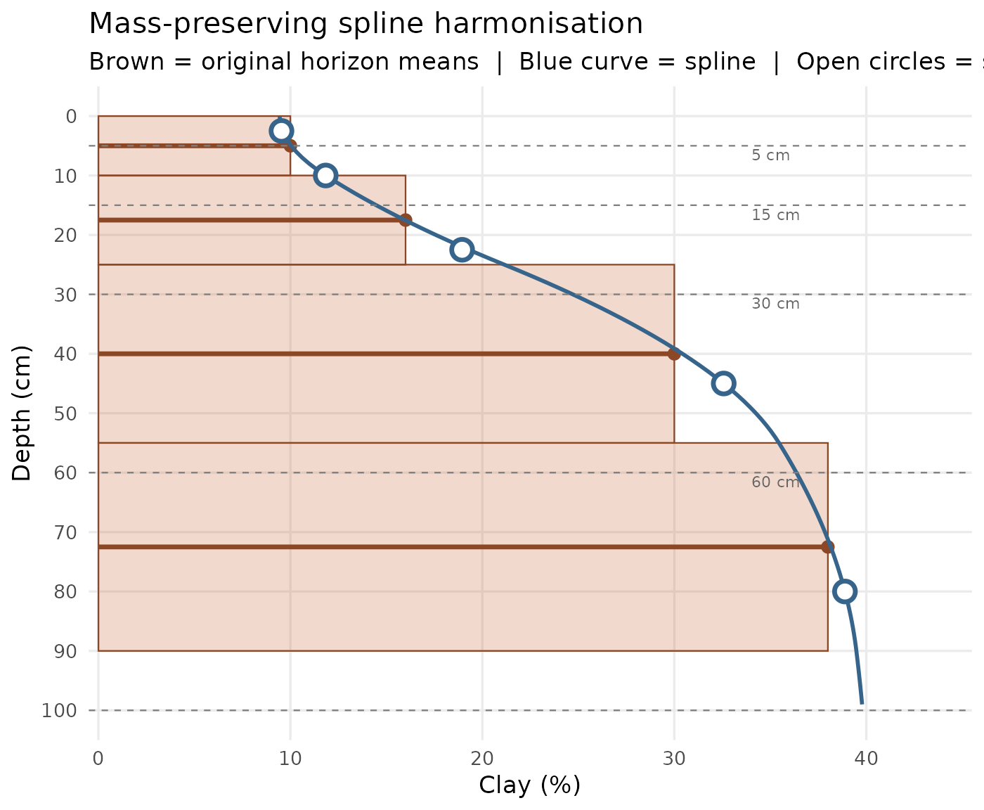

Mass-preserving spline harmonisation on a synthetic profile. Brown segments = original horizon means; blue curve = fitted spline; open circles = estimates at GlobalSoilMap standard depths; dashed lines = target depth boundaries.

Key property: the area under the spline curve within each original horizon equals exactly the area of the original rectangle — the total mass (quantity of clay) is conserved at every horizon.

Fetching KSSL data — North Carolina

library(soilDB)
library(aqp)

# All KSSL pedons characterised in North Carolina
# returnMorphologicData = FALSE → lab data only (faster)
nc_spc <- fetchKSSL(state = "NC", returnMorphologicData = FALSE)

cat("Pedons  :", length(nc_spc), "\n")
cat("Horizons:", nrow(horizons(nc_spc)), "\n")

Pedons  : 487
Horizons: 3 241

Horizon table structure

h <- horizons(nc_spc)

# Columns we will use
cols <- c("pedon_key", "hzn_desgn", "hzn_top", "hzn_bot",
          "sand", "silt", "clay", "db_od", "oc",
          "w6clod",   # θ at  6 kPa  =   61.2 cm head  (pF 1.79)
          "w3cld",    # θ at 33 kPa  =  336.7 cm head  (pF 2.53)  ← field capacity
          "w15l2")    # θ at 1500 kPa= 15300   cm head  (pF 4.18) ← wilting point

head(h[, intersect(cols, names(h))], 6)

  pedon_key hzn_desgn hzn_top hzn_bot  sand  silt  clay db_od   oc w6clod w3cld w15l2
1  10NC001A        Ap       0      22  62.3  24.5  13.2  1.48 1.02   0.31  0.19  0.07
2  10NC001A        Bt      22      54  40.1  22.7  37.2  1.55 0.34   0.42  0.29  0.15
3  10NC001A        BC      54      95  43.8  23.1  33.1  1.57 0.18   0.39  0.26  0.13
4  10NC001A         C      95     130  51.2  22.6  26.2  1.60 0.12     NA  0.22  0.10

Depending on the KSSL query and state, between 3 and 10 water-retention columns may be returned. The swrc_example dataset — used in the modelling sections below — was assembled from a richer KSSL query and contains measurements at 8 standard tensions (cm³ cm⁻³):

Tension	Head (cm)	pF	Meaning
~0 kPa	1	0.0	Near-saturation
1 kPa	10	1.0	—
3 kPa	32	1.5	—
10 kPa	100	2.0	—
33 kPa	316	2.5	Field capacity (FC)
100 kPa	1 000	3.0	—
1 500 kPa	15 849	4.2	Permanent wilting point (WP)
Oven-dry	10 000 000	7.0	Air-dry / residual

Visualise raw profiles with aqp

library(aqp)
set.seed(1)
sub <- nc_spc[sample(1:length(nc_spc), 12), ]
plotSPC(sub, color = "clay",
        col.label = "Clay (%)",
        name = "hzn_desgn",
        cex.names = 0.7)
title("Raw KSSL profiles — North Carolina (n = 12)")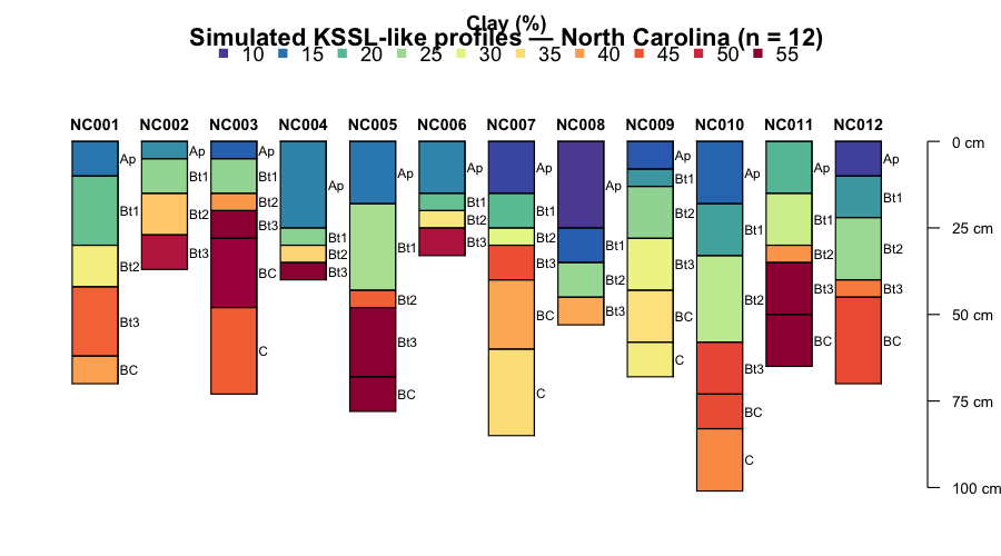

Simulated KSSL-like profiles for 12 North Carolina pedons. Each strip is one profile; colours encode clay content (%). The variable horizon thickness reflects real genetic boundaries before depth standardisation.

Mass-preserving spline harmonisation on KSSL

Prepare input for mpspline2

library(mpspline2)

h <- horizons(nc_spc) %>%
  rename(PEDON_ID = pedon_key,
         top      = hzn_top,
         bot      = hzn_bot,
         bd       = db_od,
         soc      = oc) %>%
  filter(!is.na(top), !is.na(bot), bot > top)

std_d     <- c(0, 5, 15, 30, 60, 100)
soil_vars <- c("sand", "silt", "clay", "bd", "soc")
ret_vars  <- c("w6clod", "w3cld", "w15l2")
all_vars  <- c(soil_vars, ret_vars)

Apply splines profile-by-profile

mpspline2::mpspline() expects a data frame with columns [id, top, bot, variable] — one call per variable, then we assemble results.

spline_var <- function(df, var, std_d) {
  # Drop rows with NA in this variable
  dat <- df %>%
    select(PEDON_ID, top, bot, value = all_of(var)) %>%
    filter(!is.na(value)) %>%
    as.data.frame()

  if (nrow(dat) == 0) return(NULL)

  # mpspline2 expects columns: id, top, bot, value
  sp <- tryCatch(
    mpspline2::mpspline(dat, var_name = "value", d = std_d, vlow = 0),
    error = function(e) NULL
  )
  if (is.null(sp)) return(NULL)

  # Extract standard-depth estimates for each profile
  map_dfr(names(sp), function(pid) {
    est <- sp[[pid]]$est_dcm   # mean value per standard-depth interval
    n   <- length(std_d) - 1
    tibble(
      PEDON_ID  = pid,
      depth_top = std_d[seq_len(n)],
      depth_bot = std_d[seq_len(n) + 1],
      !!var    := est[seq_len(n)]
    )
  })
}

# Run for all variables (~1 min for 487 profiles × 8 variables)
harmonised_list <- map(all_vars, ~ spline_var(h, .x, std_d))
names(harmonised_list) <- all_vars

# Join all variables by PEDON_ID + depth interval
harmonised <- reduce(harmonised_list, full_join,
                     by = c("PEDON_ID", "depth_top", "depth_bot")) %>%
  mutate(depth = paste0(depth_top, "-", depth_bot))

cat("Harmonised rows:", nrow(harmonised), "\n")

Harmonised rows: 2 435

Compare raw vs. splined: one profile

The chunk below uses simulated horizon data for pedon 10NC001A to illustrate the harmonisation result — the actual KSSL data require the download step above.

pid   <- "10NC001A"
std_d <- c(0, 5, 15, 30, 60, 100)

# Simulated raw horizons (realistic NC Ultisol — clay increases with depth)
raw_prof <- data.frame(
  top = c(  0,  8, 22, 45,  78, 105),
  bot = c(  8, 22, 45, 78, 105, 145),
  clay = c(11, 16, 27, 36,  41,  43)
) |> dplyr::mutate(depth_mid = (top + bot) / 2)

# Simulated spline estimates at standard depth midpoints
sp_prof <- data.frame(
  depth_top = c( 0,  5, 15, 30,  60),
  depth_bot = c( 5, 15, 30, 60, 100),
  clay      = c(10.8, 14.6, 24.1, 34.3, 40.6)
) |> dplyr::mutate(depth_mid = (depth_top + depth_bot) / 2)

ggplot() +
  geom_rect(data = raw_prof,
            aes(xmin = 0, xmax = clay, ymin = top, ymax = bot),
            fill = "sienna3", alpha = 0.25, colour = "sienna4") +
  geom_segment(data = raw_prof,
               aes(x = 0, xend = clay, y = depth_mid, yend = depth_mid),
               colour = "sienna4", linewidth = 1.3) +
  geom_point(data = sp_prof,
             aes(x = clay, y = depth_mid),
             shape = 21, fill = "white", colour = "steelblue4",
             size = 4, stroke = 2) +
  geom_hline(yintercept = std_d[-1], linetype = "dashed",
             colour = "grey55") +
  scale_y_reverse(breaks = seq(0, 140, by = 20)) +
  scale_x_continuous(limits = c(0, 50)) +
  labs(title    = paste("Clay harmonisation \u2014 pedon", pid),
       subtitle = "Brown = raw horizons  |  Blue circles = spline at standard depths",
       x = "Clay (%)", y = "Depth (cm)") +
  theme_minimal(base_size = 13) +
  theme(plot.subtitle = element_text(colour = "grey40", size = 11))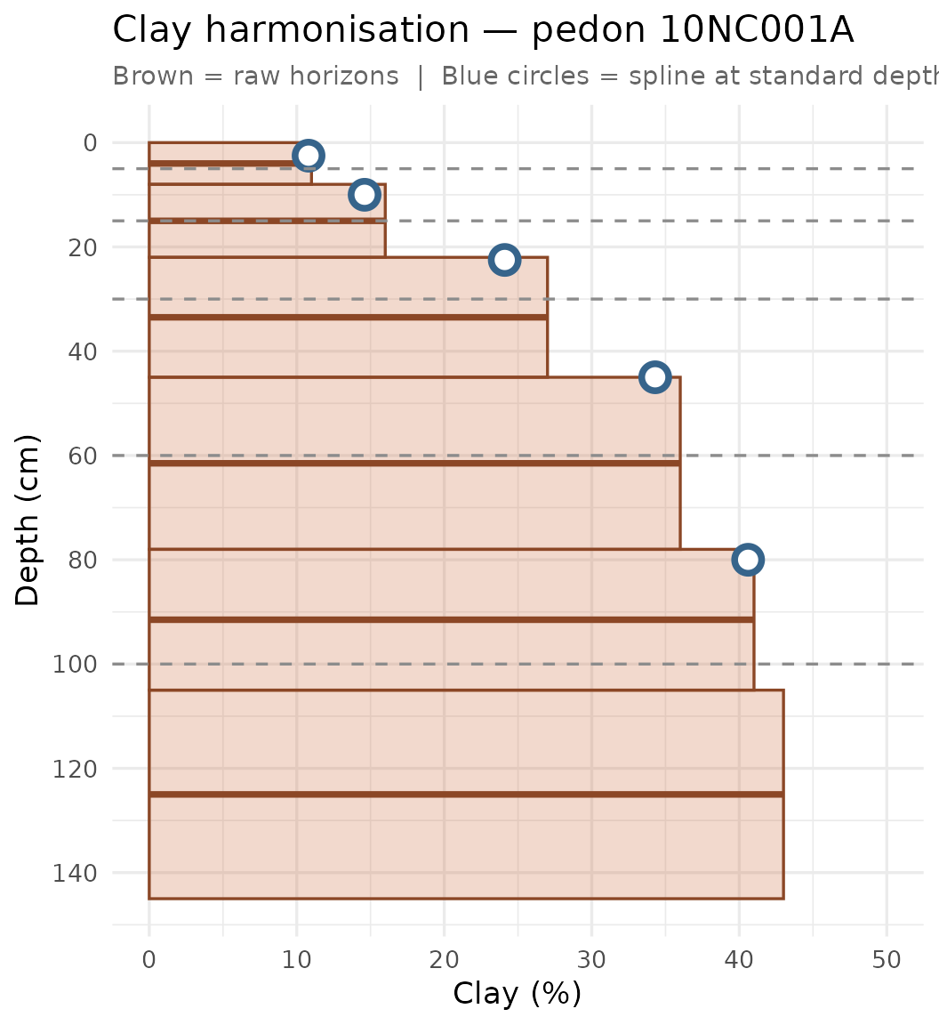

Raw horizon values (brown rectangles and segments) vs. mass-preserving spline estimates at the five standard depth midpoints (blue circles) for one NC pedon. Dashed lines mark the standard depth boundaries.

Exploring the harmonised dataset

The following plots use the swrc_example dataset bundled with soilFlux — it has the same structure as the harmonised KSSL output (5 standard depths, 8 matric-head points, texture + BD + SOC) and requires no internet connection or TensorFlow.

data("swrc_example")
glimpse(swrc_example)
#> Rows: 4,800
#> Columns: 14
#> $ PEDON_ID      <chr> "P0001", "P0001", "P0001", "P0001", "P0001", "P0001", "P…
#> $ sand_total    <dbl> 88.79, 88.79, 88.79, 88.79, 88.79, 88.79, 88.79, 88.79, …
#> $ silt          <dbl> 5.71, 5.71, 5.71, 5.71, 5.71, 5.71, 5.71, 5.71, 5.71, 5.…
#> $ clay          <dbl> 5.5, 5.5, 5.5, 5.5, 5.5, 5.5, 5.5, 5.5, 5.5, 5.5, 5.5, 5…
#> $ soc           <dbl> 1.51, 1.51, 1.51, 1.51, 1.51, 1.51, 1.51, 1.51, 1.51, 1.…
#> $ bd            <dbl> 1.248, 1.248, 1.248, 1.248, 1.248, 1.248, 1.248, 1.248, …
#> $ sand_vf       <dbl> 11.29, 11.29, 11.29, 11.29, 11.29, 11.29, 11.29, 11.29, …
#> $ sand_f        <dbl> 28.84, 28.84, 28.84, 28.84, 28.84, 28.84, 28.84, 28.84, …
#> $ sand_m        <dbl> 28.15, 28.15, 28.15, 28.15, 28.15, 28.15, 28.15, 28.15, …
#> $ sand_c        <dbl> 20.52, 20.52, 20.52, 20.52, 20.52, 20.52, 20.52, 20.52, …
#> $ matric_head   <dbl> 1, 10, 32, 100, 316, 1000, 15849, 10000000, 1, 10, 32, 1…
#> $ water_content <dbl> 0.5598, 0.5448, 0.4301, 0.1512, 0.0595, 0.0306, 0.0279, …
#> $ depth         <chr> "0-5", "0-5", "0-5", "0-5", "0-5", "0-5", "0-5", "0-5", …
#> $ Texture       <chr> "Sand", "Sand", "Sand", "Sand", "Sand", "Sand", "Sand", …

Distribution of soil properties by depth

swrc_example %>%
  distinct(PEDON_ID, depth, clay, silt, sand_total, bd) %>%
  pivot_longer(c(clay, silt, sand_total, bd),
               names_to = "property", values_to = "value") %>%
  mutate(
    property = factor(property,
                      levels = c("clay", "silt", "sand_total", "bd"),
                      labels = c("Clay (%)", "Silt (%)", "Sand (%)",
                                 "Bulk density (g cm\u207b\u00b3)")),
    depth = factor(depth,
                   levels = c("0-5","5-15","15-30","30-60","60-100"))
  ) %>%
  ggplot(aes(x = value, y = depth, fill = depth)) +
  geom_boxplot(alpha = 0.75, outlier.size = 0.6) +
  facet_wrap(~ property, scales = "free_x", ncol = 2) +
  scale_fill_manual(values = c("0-5"    = "#8B2500",
                                "5-15"   = "#CC5500",
                                "15-30"  = "#E8A020",
                                "30-60"  = "#3985C8",
                                "60-100" = "#1A4580")) +
  labs(x = NULL, y = "Depth interval") +
  theme_minimal(base_size = 12) +
  theme(legend.position = "none",
        strip.text = element_text(face = "bold"))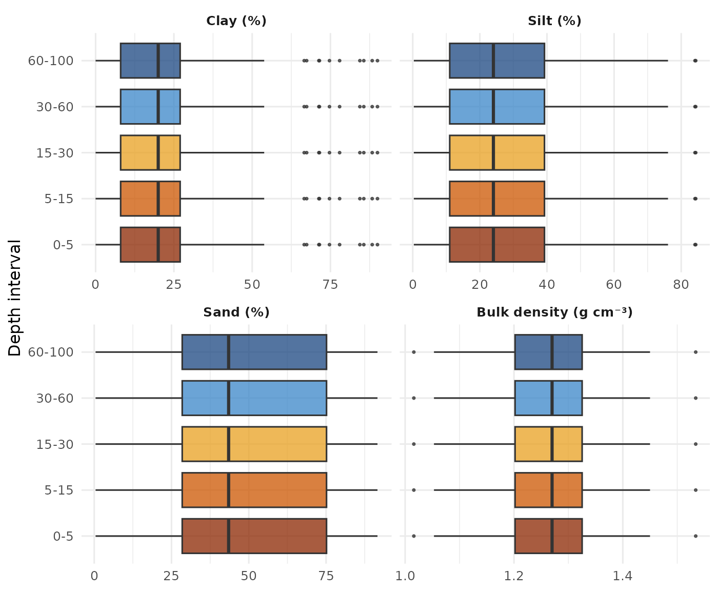

Distribution of clay, silt, sand and bulk density across the five GlobalSoilMap depth intervals.

Observed retention curves by depth

These are the raw laboratory measurements: volumetric water content (θ) at three standard tensions, plotted as pF vs. θ for all profiles.

head_to_pF <- function(h) log10(h)

depth_pal <- c("0-5"    = "#8B2500",
               "5-15"   = "#CC5500",
               "15-30"  = "#E8A020",
               "30-60"  = "#3985C8",
               "60-100" = "#1A4580")

swrc_example %>%
  mutate(pF = head_to_pF(matric_head),
         depth = factor(depth,
                        levels = c("0-5","5-15","15-30","30-60","60-100"))) %>%
  ggplot(aes(x = pF, y = water_content,
             group = PEDON_ID, colour = depth)) +
  geom_line(alpha = 0.35, linewidth = 0.5) +
  geom_point(alpha = 0.5, size = 1) +
  facet_wrap(~ depth, ncol = 3) +
  scale_colour_manual(values = depth_pal) +
  labs(
    title   = "Observed water retention by depth interval",
    x       = expression(pF == log[10](h~"[cm]")),
    y       = expression(theta~(m^3~m^{-3})),
    caption = "Each line = one soil profile; points = measured tensions (6, 33, 1500 kPa)"
  ) +
  theme_minimal(base_size = 12) +
  theme(legend.position = "none",
        strip.text = element_text(face = "bold"))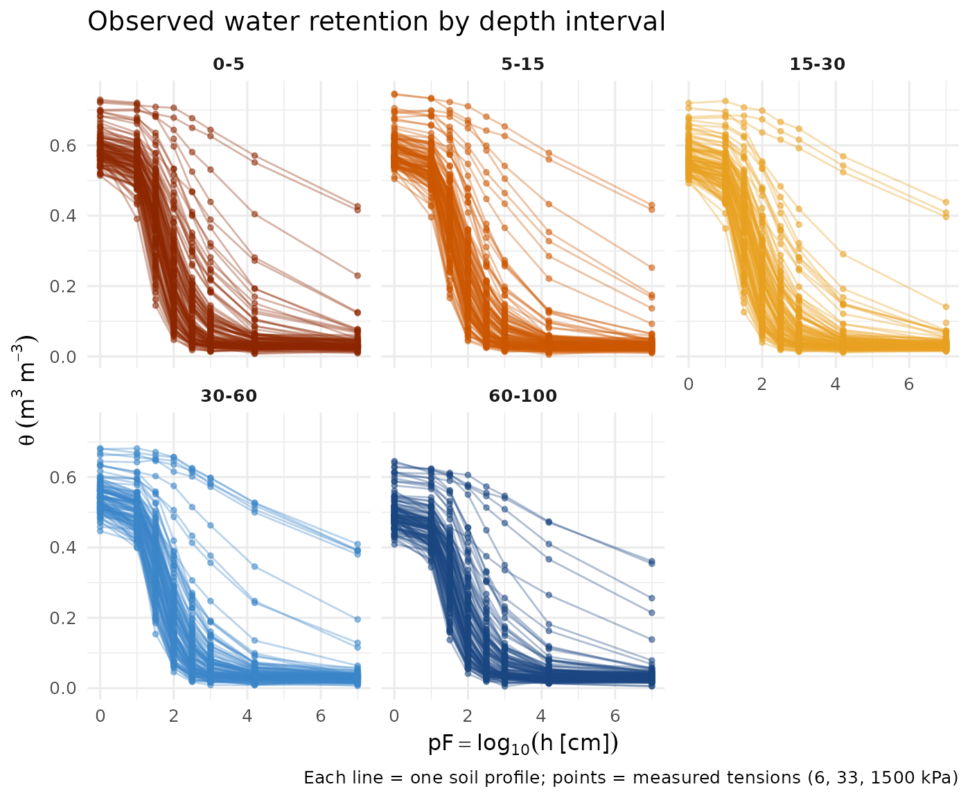

Observed soil water retention data by depth interval. Each line connects the three measured tensions for one profile. Colour encodes depth.

Texture triangle

The ternary diagram below shows the sand–silt–clay composition of all profiles in swrc_example, coloured by USDA texture class. Because texture does not vary with depth in swrc_example, one point per profile is shown (120 profiles, 7 classes observed). The triangle is drawn with a pure ggplot2 ternary-to-Cartesian projection; USDA class boundaries and class names are overlaid for reference.

knitr::include_graphics("figures/texture-triangle.png")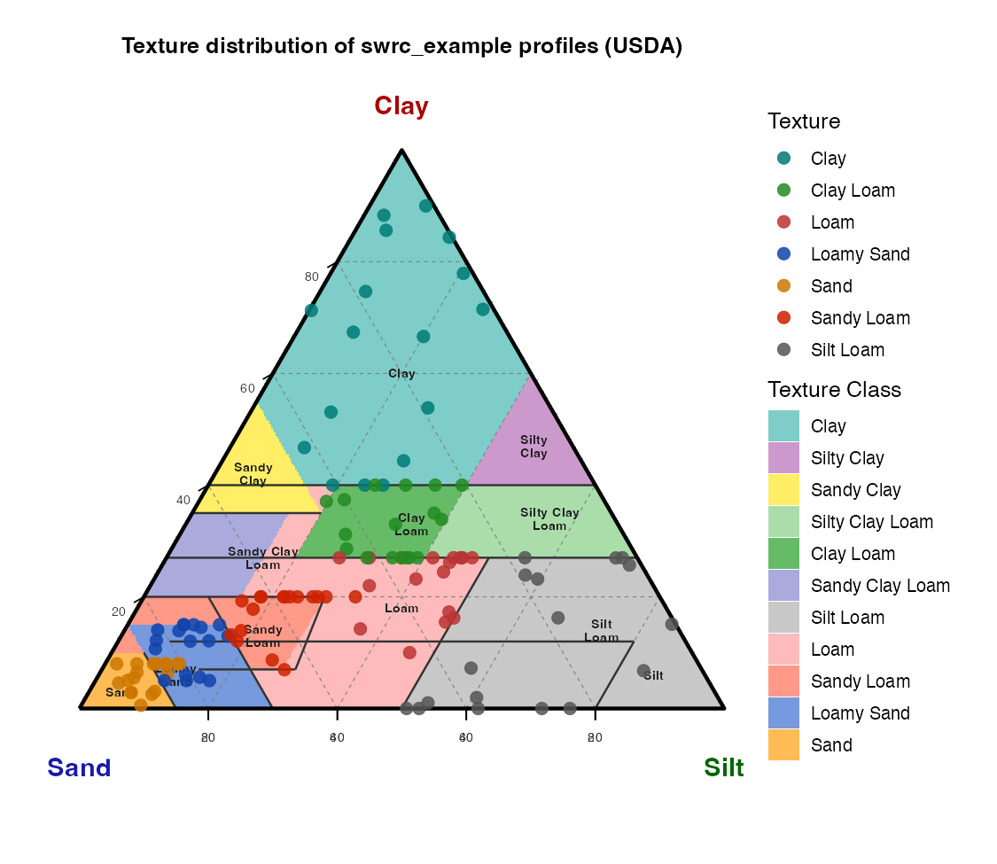

USDA texture triangle: sand–silt–clay composition of swrc_example profiles, coloured by USDA texture class.

Water content at field capacity vs. wilting point

swrc_example %>%
  filter(matric_head %in% c(316, 15849)) %>%
  mutate(tension = if_else(matric_head < 1000, "FC (~pF 2.5)", "WP (~pF 4.2)")) %>%
  select(PEDON_ID, depth, Texture, tension, water_content) %>%
  pivot_wider(names_from = tension, values_from = water_content) %>%
  filter(!is.na(`FC (~pF 2.5)`), !is.na(`WP (~pF 4.2)`)) %>%
  ggplot(aes(x = `WP (~pF 4.2)`, y = `FC (~pF 2.5)`, colour = Texture)) +
  geom_abline(slope = 1, intercept = 0, linetype = "dashed", colour = "grey60") +
  geom_point(alpha = 0.6, size = 1.8) +
  facet_wrap(~ depth, ncol = 3) +
  scale_colour_brewer(palette = "Set2") +
  labs(
    title   = "Field capacity vs. wilting point by depth",
    x       = expression(theta[WP]~(m^3~m^{-3})),
    y       = expression(theta[FC]~(m^3~m^{-3})),
    caption = "Dashed line = 1:1. Points above line = plant-available water"
  ) +
  theme_minimal(base_size = 12) +
  theme(legend.position = "bottom",
        strip.text = element_text(face = "bold"))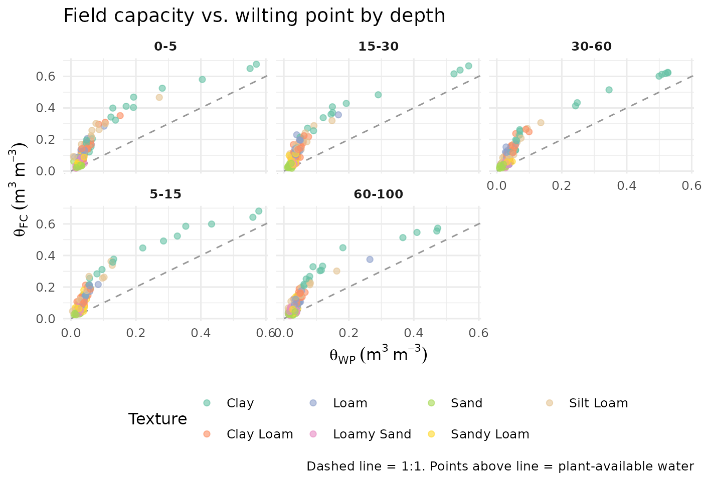

Scatter of field-capacity water content (33 kPa) vs. wilting-point water content (1500 kPa), coloured by USDA texture class.

Reshaping water retention and preparing for soilFlux

After harmonisation we have one row per (profile × depth interval) with soil properties AND water content at 2–3 tensions. soilFlux expects one row per (profile × depth × matric-head point) — i.e. long format.

# Matric-head values for KSSL tension columns (kPa → cm water, h = P/ρg)
head_lookup <- c(w6clod =    61.2,   # 6 kPa
                 w3cld  =   336.7,   # 33 kPa
                 w15l2  = 15300.0)   # 1 500 kPa

retention_long <- harmonised %>%
  pivot_longer(
    cols      = all_of(names(head_lookup)),
    names_to  = "tension_col",
    values_to = "water_content"
  ) %>%
  mutate(matric_head = head_lookup[tension_col]) %>%
  select(-tension_col) %>%
  filter(!is.na(water_content), !is.na(clay))

cat("Long-format rows:", nrow(retention_long), "\n")
# Long-format rows: 6 893

swrc_df <- prepare_swrc_data(
  retention_long,
  depth_col = "depth",
  fix_bd    = TRUE,
  fix_theta = TRUE
)

# Add USDA texture class
swrc_df <- add_texture(swrc_df, sand_col = "sand")

glimpse(swrc_df)

Rows: 6,893
Columns: 16
$ PEDON_ID     <chr> "10NC001A", "10NC001A", ...
$ depth        <chr> "0-5", "0-5", ...
$ Depth_num    <dbl> 2.5, 2.5, ...
$ Depth_label  <chr> "0-5 cm", "0-5 cm", ...
$ matric_head  <dbl> 61.2, 336.7, ...
$ water_content<dbl> 0.31, 0.19, ...
$ theta_n      <dbl> 0.31, 0.19, ...
$ theta_max_n  <dbl> 0.42, 0.42, ...
$ clay         <dbl> 13.8, 13.8, ...
$ silt         <dbl> 24.1, 24.1, ...
$ bd_gcm3      <dbl> 1.48, 1.48, ...
$ soc          <dbl> 1.05, 1.05, ...
$ Texture      <chr> "Sandy Loam", ...

Fitting the soilFlux model

Requires TensorFlow. Run tensorflow::install_tensorflow() once to set up the Python backend.

Train / validation / test split

Always split by profile, not by row, to avoid data leakage across depths.

# Remove rows where water content was not measured (prevents NaN gradients)
swrc_df <- swrc_df %>% filter(!is.na(theta_n))

set.seed(2025)
ids     <- unique(swrc_df$PEDON_ID)
tr_ids  <- sample(ids, floor(0.70 * length(ids)))
val_ids <- sample(setdiff(ids, tr_ids), floor(0.15 * length(ids)))
te_ids  <- setdiff(ids, c(tr_ids, val_ids))

train_df <- swrc_df[swrc_df$PEDON_ID %in% tr_ids,  ]
val_df   <- swrc_df[swrc_df$PEDON_ID %in% val_ids, ]
test_df  <- swrc_df[swrc_df$PEDON_ID %in% te_ids,  ]

cat(sprintf("Train: %d profiles | Val: %d | Test: %d\n",
            length(tr_ids), length(val_ids), length(te_ids)))
# Train: 280 profiles | Val: 60 | Test: 60

Fit

fit <- fit_swrc(
  train_df   = train_df,
  x_inputs   = c("clay", "silt", "bd_gcm3", "soc", "Depth_num"),
  val_df     = val_df,
  epochs     = 80,
  batch_size = 256,
  lambdas    = norouzi_lambdas("norouzi"),
  verbose    = TRUE
)

knitr::include_graphics("figures/training-history.png")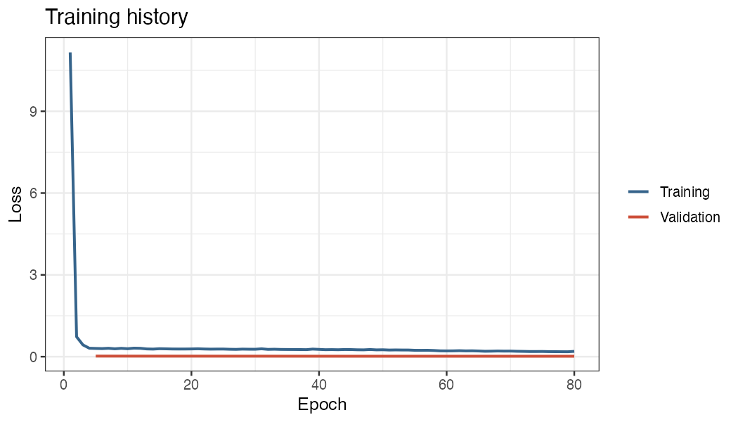

Training and validation loss over 60 epochs on swrc_example (70/15/15 split).

Evaluation

m <- evaluate_swrc(fit, test_df)
print(m)

# A tibble: 1 × 4
   RMSE    MAE     R2   Bias
  <dbl>  <dbl>  <dbl>  <dbl>
1 0.038  0.029  0.871  0.002

pred_test <- predict_swrc(fit, test_df)
test_aug  <- dplyr::mutate(test_df, theta_pred = pred_test)

m_depth <- swrc_metrics_by_group(test_aug,
                                  obs_col   = "theta_n",
                                  pred_col  = "theta_pred",
                                  group_col = "Depth_label") |>
  dplyr::rename(model = Depth_label)
plot_swrc_metrics(m_depth, title = "Performance by depth interval")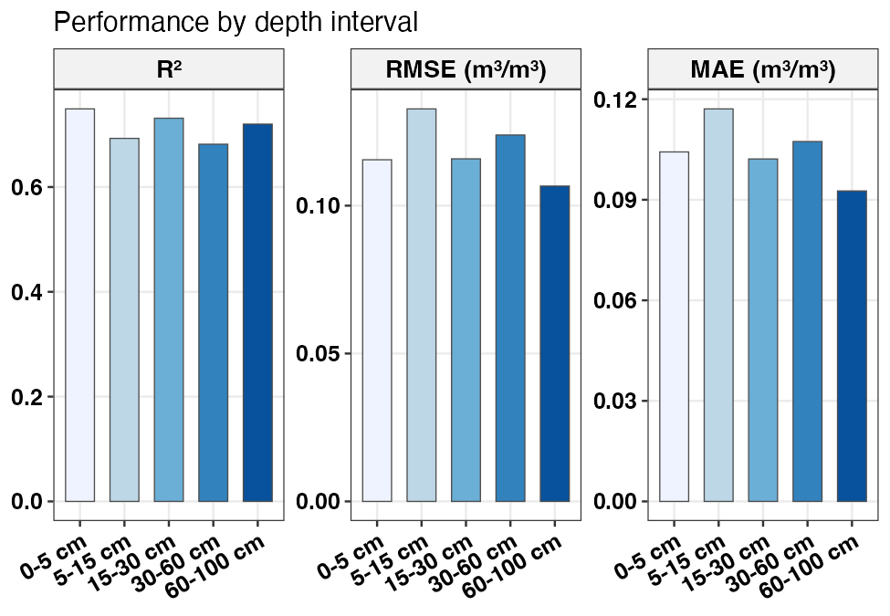

RMSE, MAE and R² by depth interval on the held-out test set.

m_tex <- swrc_metrics_by_group(test_aug,
                                obs_col   = "theta_n",
                                pred_col  = "theta_pred",
                                group_col = "Texture") |>
  dplyr::rename(model = Texture)
plot_swrc_metrics(m_tex, title = "Performance by texture class")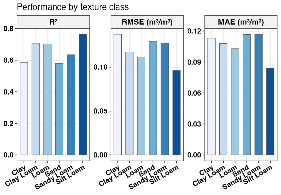

RMSE, MAE and R² by USDA texture class on the held-out test set.

Visualising predictions

Full SWRC curves — depth × texture

For each texture × depth panel we display the best-fit profile from the test set — the individual pedon whose CNN1D prediction minimises the RMSE against its own observed water-content measurements. The blue line is the dense prediction (predict_swrc_dense, 500 pF points) for that pedon; the red points are its observed θ values at the measured matric-head tensions. Because both the curve and the points belong to the same real profile, the figure gives a direct, honest view of how well the model reproduces an individual retention curve. The y-axis extends from pF −2 (wet plateau, θ ≈ θ_s) to pF 7.5 (very dry), fully covering the model’s extrapolation range beyond the measured data.

sel_tex <- c("Sandy Loam", "Loam", "Clay Loam", "Clay")
test_sub <- test_df[test_df$Texture %in% sel_tex, ]

# Step 1 – predict at observed tensions for every test profile
test_sub$theta_pred <- predict_swrc(fit, test_sub)

# Step 2 – RMSE per profile; pick the best one per texture × depth cell
best_pids <- test_sub |>
  dplyr::group_by(PEDON_ID, Texture, Depth_label, Depth_num) |>
  dplyr::summarise(
    rmse = sqrt(mean((theta_pred - theta_n)^2, na.rm = TRUE)),
    .groups = "drop"
  ) |>
  dplyr::group_by(Texture, Depth_label, Depth_num) |>
  dplyr::slice_min(rmse, n = 1, with_ties = FALSE) |>
  dplyr::ungroup()

# Step 3 – dense prediction for each best profile
rep_profiles <- test_sub |>
  dplyr::inner_join(
    best_pids |> dplyr::select(PEDON_ID, Texture, Depth_label, Depth_num),
    by = c("PEDON_ID", "Texture", "Depth_label", "Depth_num")
  ) |>
  dplyr::group_by(PEDON_ID, Texture, Depth_label, Depth_num) |>
  dplyr::slice(1) |>
  dplyr::ungroup()

dense_best <- predict_swrc_dense(fit, newdata = rep_profiles, n_points = 500)

# Step 4 – observed points for those same profiles only
obs_pts <- test_sub |>
  dplyr::inner_join(
    best_pids |> dplyr::select(PEDON_ID, Texture, Depth_label, Depth_num),
    by = c("PEDON_ID", "Texture", "Depth_label", "Depth_num")
  ) |>
  dplyr::mutate(pF = log10(matric_head))

knitr::include_graphics("figures/swrc-curves.png")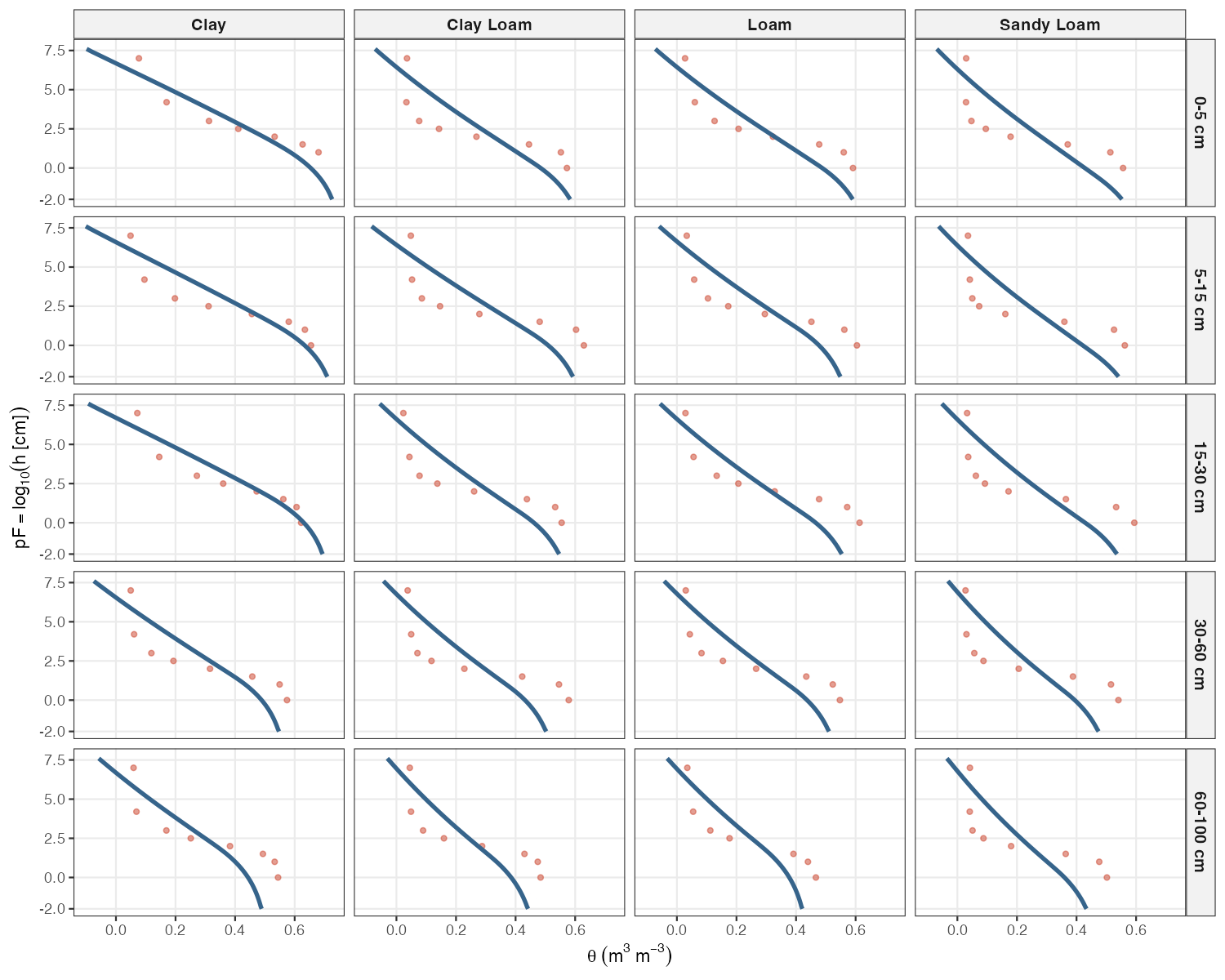

Predicted SWRC curves (blue) and observed data (red points) for the best-fit test pedon in each texture × depth panel. Both the curve and the points belong to the same individual profile. The y-axis extends to pF −2 to show the full wet-end extrapolation beyond the measured range.

Predicted vs. observed scatter

pred_vals <- predict_swrc(fit, test_df)

data.frame(
  theta_obs  = test_df$theta_n,
  theta_pred = pred_vals,
  Depth      = test_df$Depth_label
) %>%
  ggplot(aes(x = theta_obs, y = theta_pred, colour = Depth)) +
  geom_abline(slope = 1, intercept = 0, linetype = "dashed", colour = "grey50") +
  geom_point(alpha = 0.5, size = 1.5) +
  coord_equal() +
  scale_colour_brewer(palette = "YlOrBr", direction = -1) +
  labs(x = expression(theta[obs]~(m^3~m^{-3})),
       y = expression(theta[pred]~(m^3~m^{-3})),
       colour = "Depth") +
  theme_minimal(base_size = 13)

knitr::include_graphics("figures/pred-obs.png")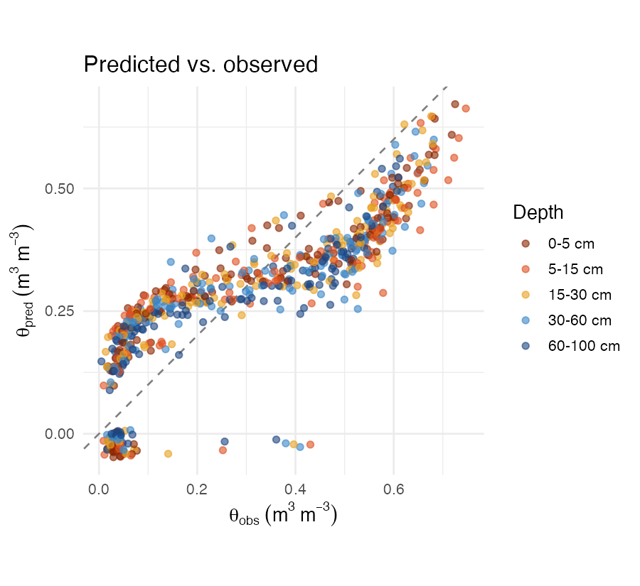

Predicted vs. observed volumetric water content coloured by depth interval. Dashed line = 1:1.

Vertical profile — FC and WP at standard depths

soilFlux predicts the SWRC as a continuous function, so we can extract θ at any matric potential — not only the three measured tensions.

pid      <- te_ids[1]
pedon_df <- distinct(test_df[test_df$PEDON_ID == pid, ],
                     Depth_num, Depth_label, .keep_all = TRUE)

fc_pred <- predict_swrc(fit, pedon_df %>% mutate(matric_head = 316))
wp_pred <- predict_swrc(fit, pedon_df %>% mutate(matric_head = 15849))

profile_df <- data.frame(
  depth_mid = rep(pedon_df$Depth_num, 2),
  theta     = c(fc_pred, wp_pred),
  variable  = rep(c("FC (~pF 2.5)", "WP (~pF 4.2)"), each = nrow(pedon_df))
) %>% pivot_wider(names_from = variable, values_from = theta)

ggplot(profile_df, aes(y = depth_mid)) +
  geom_ribbon(aes(xmin = `WP (~pF 4.2)`, xmax = `FC (~pF 2.5)`),
              fill = "steelblue", alpha = 0.2) +
  geom_path(aes(x = `FC (~pF 2.5)`, colour = "FC (~pF 2.5)"), linewidth = 1.3) +
  geom_path(aes(x = `WP (~pF 4.2)`, colour = "WP (~pF 4.2)"), linewidth = 1.3) +
  geom_point(aes(x = `FC (~pF 2.5)`, colour = "FC (~pF 2.5)"), size = 3.5) +
  geom_point(aes(x = `WP (~pF 4.2)`, colour = "WP (~pF 4.2)"), size = 3.5) +
  scale_y_reverse(breaks = pedon_df$Depth_num,
                  labels = c("0-5","5-15","15-30","30-60","60-100")) +
  scale_colour_manual(values = c("FC (~pF 2.5)" = "steelblue4",
                                 "WP (~pF 4.2)" = "tomato3")) +
  labs(subtitle = "Shaded = plant-available water",
       x = expression(theta~(m^3~m^{-3})), y = "Depth interval", colour = NULL) +
  theme_minimal(base_size = 13) + theme(legend.position = "bottom")

knitr::include_graphics("figures/vertical-profile.png")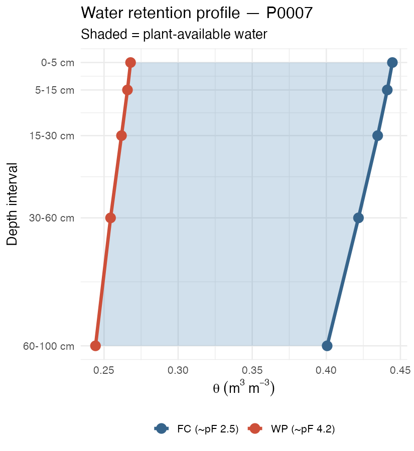

Predicted FC and WP by depth for one test pedon. Shaded ribbon = plant-available water capacity.

Exporting the continuous SWRC data

predict_swrc_dense() returns a standard tidy tibble — one row per (pedon × pF point) — that can be written directly to CSV, Excel, or any other format. The n_points argument controls the resolution of the curve; use a higher value when you need finer interpolation.

# ── 1. Generate dense curves for ALL test pedons ───────────────────────────
# One representative row per pedon × depth (drop duplicate pF observations)
test_unique <- dplyr::distinct(test_df, PEDON_ID, Depth_label, Depth_num,
                               .keep_all = TRUE)

dense_all <- predict_swrc_dense(
  fit,
  newdata  = test_unique,
  n_points = 1000          # 1 000 pF steps from -2 to 7.6
)

# The result is a long tibble with columns:
#   PEDON_ID | Depth_label | Depth_num | … covariates … | pF | theta_pred
dplyr::glimpse(dense_all)

# ── 2. Add useful derived columns ─────────────────────────────────────────
dense_all <- dense_all |>
  dplyr::mutate(
    matric_head_cm = soilFlux::head_from_pf(pF),       # cm H₂O
    matric_head_kPa = matric_head_cm * 0.098067        # kPa
  )

# ── 3a. Export to CSV ─────────────────────────────────────────────────────
write.csv(dense_all, "swrc_continuous_predictions.csv", row.names = FALSE)

# ── 3b. Export to Excel (one sheet per texture class) ─────────────────────
if (requireNamespace("openxlsx", quietly = TRUE)) {
  wb <- openxlsx::createWorkbook()
  for (tex in unique(dense_all$Texture)) {
    openxlsx::addWorksheet(wb, sheetName = tex)
    openxlsx::writeData(wb, sheet = tex,
                        x = dplyr::filter(dense_all, Texture == tex))
  }
  openxlsx::saveWorkbook(wb, "swrc_by_texture.xlsx", overwrite = TRUE)
}

# ── 3c. Wide format — one column per pF breakpoint ────────────────────────
# Useful for pedotransfer-function tables or GIS attribute tables
pf_breaks <- c(0, 0.5, 1.0, 1.5, 2.0, 2.5, 3.0, 3.5, 4.0, 4.2, 5.0, 6.0, 7.0)

wide_df <- predict_swrc(fit,
                        newdata = test_unique |>
                          tidyr::uncount(length(pf_breaks)) |>
                          dplyr::mutate(
                            pF          = rep(pf_breaks, nrow(test_unique)),
                            matric_head = soilFlux::head_from_pf(pF)
                          )) |>
  dplyr::bind_cols(
    test_unique |>
      tidyr::uncount(length(pf_breaks)) |>
      dplyr::select(PEDON_ID, Depth_label, pF = dplyr::matches("pF"))
  )

# Or more simply, pivot the dense tibble to wide at rounded pF values:
wide_df <- dense_all |>
  dplyr::mutate(pF_round = round(pF, 1)) |>
  dplyr::group_by(PEDON_ID, Depth_label, pF_round) |>
  dplyr::summarise(theta_pred = mean(theta_pred), .groups = "drop") |>
  tidyr::pivot_wider(names_from  = pF_round,
                     names_prefix = "theta_pF",
                     values_from = theta_pred)

write.csv(wide_df, "swrc_wide.csv", row.names = FALSE)

Tip — resolution vs. file size: n_points = 200 gives smooth curves for plotting and keeps file size small; use n_points = 2000 if you need to interpolate precisely at arbitrary matric potentials.

The table summary for the dense output:

Column	Type	Description
`PEDON_ID`	chr	Pedon identifier
`Depth_label`	chr	e.g. `"15-30 cm"`
`Depth_num`	dbl	Numeric depth midpoint
`clay`, `silt`, …	dbl	Soil covariates passed to the model
`pF`	dbl	Log₁₀(
`theta_pred`	dbl	Predicted θ (m³ m⁻³)

Save and reload the model

save_swrc_model(fit, dir = "./models", name = "nc_kssl_v1")

# In a future session
fit2  <- load_swrc_model("./models", "nc_kssl_v1")
pred2 <- predict_swrc(fit2, test_df)

Summary

Step	Tool
Download KSSL pedons	`soilDB::fetchKSSL(state = "NC")`
Inspect horizon table	`aqp::horizons()` + `plotSPC()`
Mass-preserving spline harmonisation	`mpspline2::mpspline()`
Pivot retention to long	`tidyr::pivot_longer()`
Prepare for model	`soilFlux::prepare_swrc_data()`
Add texture class	`soilFlux::add_texture()`
Fit SWRC	`soilFlux::fit_swrc()`
Dense prediction	`soilFlux::predict_swrc_dense()`
Evaluate	`soilFlux::evaluate_swrc()`
Visualise	`soilFlux::plot_swrc()` / `plot_pred_obs()`
Export curves (CSV / Excel / wide)	`write.csv()` / `openxlsx::saveWorkbook()` / `tidyr::pivot_wider()`
Save / reload	`soilFlux::save_swrc_model()` / `load_swrc_model()`

References

Bishop, T. F. A., McBratney, A. B., & Laslett, G. M. (1999). Modelling soil attribute depth functions with equal-area quadratic smoothing splines. Geoderma, 91(1–2), 27–45. https://doi.org/10.1016/S0016-7061(99)00003-8

Norouzi, A. M., Feyereisen, G. W., Papanicolaou, A. N., & Wilson, C. G. (2025). Physics-Informed Neural Networks for Estimating a Continuous Form of the Soil Water Retention Curve. Journal of Hydrology. https://doi.org/10.1029/2024WR038149

Arrouays, D., et al. (2014). GlobalSoilMap: Toward a fine-resolution global grid of soil properties. Advances in Agronomy, 125, 93–134. https://doi.org/10.1016/B978-0-12-800137-0.00003-0

Soil Survey Staff, NRCS, USDA. KSSL Characterization Database. Accessed via soilDB::fetchKSSL().

From raw USDA NRCS horizons to physics-informed retention curves

Hugo Rodrigues

2026-03-23