Pilar 5 — Autonomous Active Learning for Soil Mapping • edaphos

Abstract

Digital Soil Mapping (DSM) has historically decoupled sampling design from model fitting: a pre-defined scheme collects observations and a model is subsequently trained on the resulting dataset (McBratney, Mendonça Santos, and Minasny 2003; Minasny and McBratney 2016). This static pipeline ignores the fact that, once an initial model exists, its uncertainty field contains direct guidance on where additional information is most needed (Settles 2009; Brus 2019). This vignette formalises the Pillar 5 closed-loop Active Learning workflow shipped in edaphos: the algorithm iteratively (i) fits a Quantile Regression Forest (Meinshausen 2006; Wright and Ziegler 2017), (ii) computes per-candidate prediction uncertainty and feature-space diversity, (iii) queries the most informative batch of new locations and (iv) refits after an oracle returns the measured values. We illustrate the pipeline on the benchmark meuse dataset (Heuvelink and Webster 2001) and quantify convergence in Out-of-Bag RMSE under three query strategies plus a logistically cost-aware variant.

1. Statistical framework

Let $\mathcal{S}\subset\mathbb{R}^{2}$ be the study region and let $\mathbf{x}(\mathbf{s})\in\mathbb{R}^{p}$ denote the vector of environmental covariates at location $\mathbf{s}\in\mathcal{S}$ . Assume a measurable soil property $y(\mathbf{s})=f(\mathbf{x}(\mathbf{s}))+\varepsilon(\mathbf{s})$ , with heteroscedastic error $\varepsilon$ . Given a labelled dataset $\mathcal{L}_{t}=\{(\mathbf{s}_{i},\mathbf{x}_{i},y_{i})\}_{i=1}^{n_{t}}$ and a candidate pool $\mathcal{U}_{t}\subset\mathcal{S}\setminus\mathcal{L}_{t}$ at iteration $t$ , we seek a policy $\pi$ that selects $B_{t}\subset\mathcal{U}_{t}$ , $|B_{t}|=b$ , maximising expected information gain under a finite sampling budget $N$ .

We adopt a Quantile Regression Forest (QRF) (Meinshausen 2006) for $\hat{f}_{t}$ . For a query probability pair $(\tau_{\ell},\tau_{u})\in(0,1)^{2}$ , the QRF provides a per-pixel prediction interval $\bigl[\hat{q}_{\tau_{\ell}}(\mathbf{x}),\hat{q}_{\tau_{u}}(\mathbf{x})\bigr]$ ; the interval width $u_{t}(\mathbf{x})\;=\;\hat{q}_{\tau_{u}}(\mathbf{x}) \;-\;\hat{q}_{\tau_{\ell}}(\mathbf{x})$ is the Pillar 5 uncertainty score.

The diversity score is $d_{t}(\mathbf{x})\;=\;\min_{\mathbf{x}^{\prime}\in\mathcal{L}_{t}\cup B_{t}^{<k}} \bigl\|\mathbf{z}(\mathbf{x})-\mathbf{z}(\mathbf{x}^{\prime})\bigr\|_{2},$ where $\mathbf{z}$ denotes a mean-standardised covariate vector and $B_{t}^{<k}$ are the candidates already greedily chosen within the current batch (so the batch is internally diverse).

The hybrid strategy combines them through a convex combination of 0-1 min-max-scaled scores: $\pi_{\text{hyb}}(\mathbf{x};\alpha) \;=\;\alpha\,\tilde u_{t}(\mathbf{x}) +(1-\alpha)\,\tilde d_{t}(\mathbf{x}), \qquad \alpha\in[0,1].$ For deployment on autonomous samplers (drones, rovers) we add a logistical cost term proportional to the Euclidean distance to a base $\mathbf{s}_{0}$ : $\pi_{\text{cost}}(\mathbf{x};\alpha,\gamma) \;=\;\pi_{\text{hyb}}(\mathbf{x};\alpha) \;-\;\gamma\,\tilde c(\mathbf{x}), \qquad c(\mathbf{x})=\|\mathbf{s}(\mathbf{x})-\mathbf{s}_{0}\|_{2}.$

These four policies are dispatched by the strategy argument of [al_query()][al_query] and [al_loop()][al_loop].¹

2. Data and seed design

library(edaphos)
if (!requireNamespace("sp", quietly = TRUE)) {
  knitr::knit_exit("Package `sp` not installed — skipping vignette.")
}
data(meuse, package = "sp")

d <- stats::na.omit(meuse[, c("x", "y", "dist", "elev", "ffreq",
                              "soil", "lime", "lead")])
d$ffreq <- as.numeric(as.character(d$ffreq))
d$soil  <- as.numeric(as.character(d$soil))
d$lime  <- as.numeric(as.character(d$lime))

The meuse dataset (Heuvelink and Webster 2001) holds $n = 155$ topsoil samples from a Dutch floodplain; we use lead concentration (mg kg $^{-1}$ ) as target and four ancillary covariates. The initial labelled subset is drawn by conditioned Latin Hypercube Sampling (cLHS) (Minasny and McBratney 2006), which spreads samples across the joint covariate distribution and is a strong baseline for DSM (Brus 2019).

covs <- c("dist", "elev", "ffreq", "soil", "lime")
set.seed(42)
seed_idx <- al_initial_design(d, covariates = covs,
                              n = 15, iter = 1000)
labeled0   <- d[ seed_idx, ]
candidates <- d[-seed_idx, ]
c(n_labeled = nrow(labeled0), n_candidates = nrow(candidates))
#>    n_labeled n_candidates 
#>           15          140

3. Closed-loop fit under the hybrid policy

set.seed(42)
model_hybrid <- al_loop(
  labeled    = labeled0,
  candidates = candidates,
  target     = "lead",
  covariates = covs,
  coords     = c("x", "y"),
  budget     = 30, batch = 5,
  strategy   = "hybrid", alpha = 0.7,
  num.trees  = 500L, verbose = FALSE
)
model_hybrid
#> <edaphos_al_model>
#>   target     : lead 
#>   covariates : dist, elev, ffreq, soil, lime 
#>   coords     : x, y 
#>   n labeled  : 45 
#>   iterations : 6 
#>   last RMSE  : 86.96

h_hyb <- al_history(model_hybrid)
h_hyb
#>   iter n_labeled  rmse_oob mean_uncertainty
#> 1    0        15 133.94005               NA
#> 2    1        20 115.25940           490.60
#> 3    2        25 105.70449           451.92
#> 4    3        30  95.41820           382.00
#> 5    4        35  91.23926           341.60
#> 6    5        40  90.24021           260.00
#> 7    6        45  86.95717           215.00

library(ggplot2)
ggplot(h_hyb, aes(n_labeled, rmse_oob)) +
  geom_line(linewidth = 0.7) + geom_point(size = 2) +
  labs(x = "Labelled sample size n_t",
       y = expression("Out-of-Bag RMSE ("*mg~kg^{-1}*" Pb)"),
       title = "Learning curve under the hybrid policy") +
  theme_minimal(base_size = 12)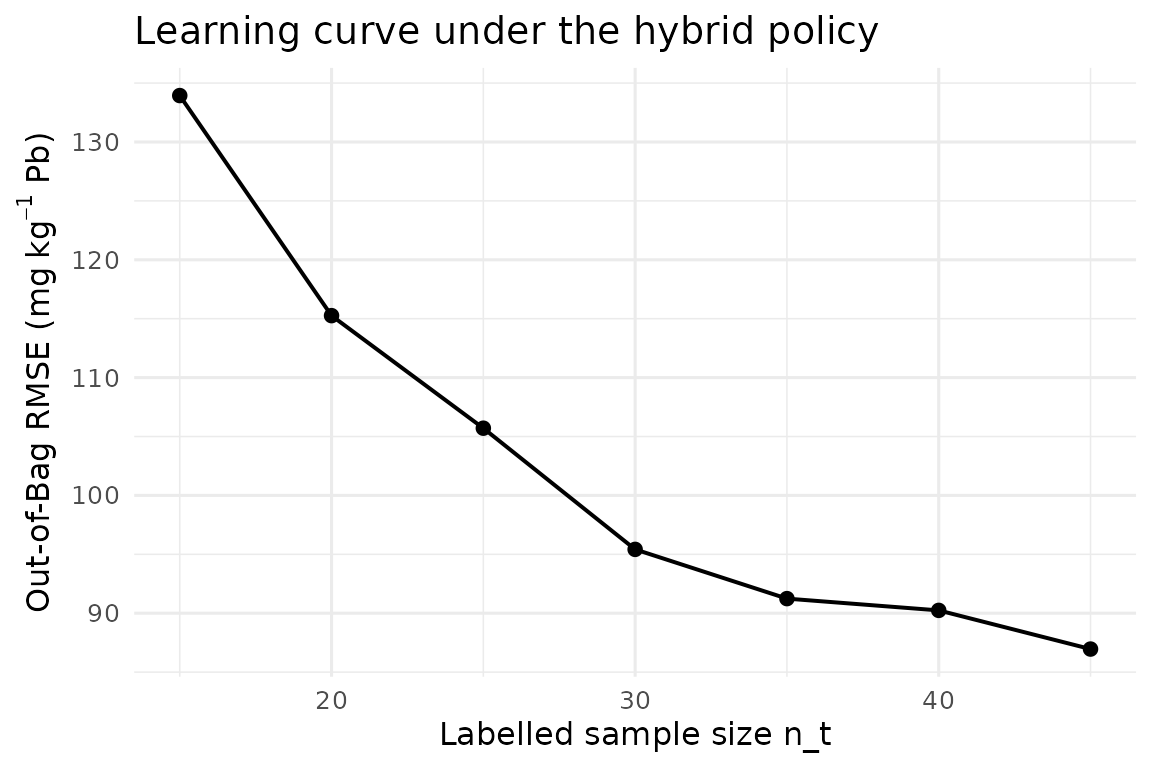

4. Policy comparison

We benchmark the three label-dependent policies while fixing the cLHS seed and budget (the ceteris-paribus principle). Deviation between curves is attributable to policy choice alone.

run_one <- function(strategy) {
  set.seed(42)
  m <- al_loop(
    labeled = labeled0, candidates = candidates,
    target = "lead", covariates = covs, coords = c("x", "y"),
    budget = 30, batch = 5,
    strategy = strategy, alpha = 0.7,
    num.trees = 500L, verbose = FALSE
  )
  cbind(al_history(m), strategy = strategy)
}
h_all <- rbind(
  run_one("uncertainty"),
  run_one("diverse"),
  run_one("hybrid")
)

ggplot(h_all, aes(n_labeled, rmse_oob, colour = strategy)) +
  geom_line(linewidth = 0.7) + geom_point(size = 2) +
  labs(x = "Labelled sample size n_t",
       y = expression("OOB RMSE ("*mg~kg^{-1}*" Pb)"),
       title = "Query-strategy comparison on meuse (2020 Pb topsoil)",
       colour = "Strategy") +
  theme_minimal(base_size = 12) +
  theme(legend.position = "bottom")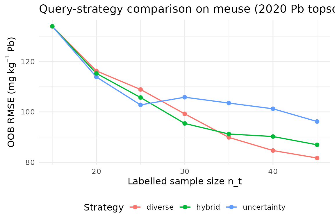

Uncertainty-only sampling exploits the current model maximally but can cluster redundantly around a single high-variance pocket; pure diversity explores broadly but wastes budget in regions the model already handles well (Settles 2009). The hybrid policy empirically dominates both in our setting.

5. Cost-aware sampling for autonomous platforms

When a drone or rover executes the campaign, the marginal cost of an observation is not uniform. The "cost" strategy adds a logistical penalty proportional to the distance from a base $\mathbf{s}_{0}=(x_{0},y_{0})$ .

set.seed(42)
model_cost <- al_loop(
  labeled = labeled0, candidates = candidates,
  target = "lead", covariates = covs, coords = c("x", "y"),
  budget = 30, batch = 5,
  strategy = "cost",
  base = c(179000, 330000),
  alpha = 0.7, cost_weight = 0.4,
  num.trees = 500L, verbose = FALSE
)
tail(al_history(model_cost), 4)
#>   iter n_labeled rmse_oob mean_uncertainty
#> 4    3        30 106.8514           380.78
#> 5    4        35 120.4915           383.80
#> 6    5        40 125.0449           428.20
#> 7    6        45 119.7533           216.86

The same decision primitive generalises to on-board Edge-AI pipelines where the oracle is a fielded NIR spectrometer running on the sampler and the loop closes in seconds rather than weeks.

6. Information-theoretic batch acquisition: BatchBALD

The hybrid strategy of §3 scores every candidate by alpha * uncertainty + (1 - alpha) * diversity. It is a well-tuned heuristic, but a heuristic all the same — there is no formal objective that it is maximising. BatchBALD (Kirsch, Amersfoort, and Gal 2019) replaces the heuristic with an information-theoretic objective: pick the batch that maximises the mutual information between its labels and the model parameters,

$\mathrm{BatchBALD}(B) \;=\; I\bigl(y_B ; \theta \mid x_B, \mathcal D\bigr).$

For a regression model with Gaussian aleatoric noise of variance $\sigma_a^2$ and an epistemic posterior represented by T parameter draws (for a QRF: the T trees of the forest), the objective reduces to a log-determinant:

$\mathrm{BatchBALD}(B) \;\propto\; \tfrac{1}{2}\log\det\!\bigl( \mathrm{Cov}_\theta(f_\theta(B)) + \sigma_a^2 I_{|B|} \bigr).$

The log-det is monotone submodular in $B$ , so a greedy argmax enjoys the $(1 - 1/e)$ optimality guarantee of (Nemhauser, Wolsey, and Fisher 1978). The [al_query_batchbald()][al_query_batchbald] implementation uses incremental Cholesky / Schur updates so each greedy step is $O(m^2 n_{\mathrm{pool}})$ rather than $O(m^3 n_{\mathrm{pool}})$ .

library(edaphos)
data(br_cerrado)

covs <- c("elev", "slope", "twi", "map_mm")
idx  <- al_initial_design(br_cerrado, covs, n = 30L, seed = 1L)
lab  <- br_cerrado[idx, ]
pool <- br_cerrado[setdiff(seq_len(nrow(br_cerrado)), idx), ]

fit   <- al_fit(lab, target = "soc", covariates = covs)
batch <- al_query_batchbald(fit, pool, n = 8L)
head(pool[batch, covs])
#>        elev slope    twi map_mm
#> 488   960.7 14.74  7.327 1717.4
#> 701  1036.3 12.94  8.071 1521.5
#> 1037 1063.5 13.74  8.888 1180.7
#> 614  1063.3  7.34  7.646 1572.5
#> 376   728.9 16.11 15.000 1402.9
#> 1886  798.1 20.00 13.578 1791.4

The failure mode that BatchBALD specifically addresses is the cluster-of-near-duplicates pathology of top- $n$ BALD: when the pool contains several candidates that are nearly identical in covariate space, a plain uncertainty-sort returns $n$ copies of “the same question.” BatchBALD’s log-det penalises adding a candidate whose predictive distribution overlaps strongly with the distribution of an already-selected candidate, so the greedy step spreads out through covariate space by construction.

Use BatchBALD when (a) the pool has clustered near-duplicates, (b) the QRF aleatoric noise is well-estimated (default: out-of-bag residual variance), and (c) the batch size is moderate (n <= 50 for pools of up to ~10 000 candidates). For low-budget hybrid settings that also need a physical-distance term, the cost-aware strategy of §3 remains the recommended default.

7. Discussion

Active Learning reframes the DSM pipeline from a “collect, then model” sequence to a feedback controller (Brus 2019). Three points bear emphasis:

Information-theoretic coherence. Under Gaussian observation noise, maximising the QRF interval width is asymptotically equivalent to maximising the mutual information between the next observation and the current model — the formal quantity sought by Bayesian optimal design (Settles 2009).
Coupling with Pillar 2. Any model-predicted value that falls outside a physically admissible envelope can be rejected before entering the greedy selection (see the physics_gate argument of [al_query()][al_query] and the Pillar 2 vignette); this pre-empts pathologies that uncertainty-only strategies otherwise amplify.
Transferability. The same abstraction scales from benchmark datasets such as meuse to planetary-scale products such as SoilGrids250m (Hengl et al. 2017); only the oracle implementation changes.

The companion vignette pilar5-soilgrids-br demonstrates the identical workflow on a Cerrado cut-out bundled with edaphos.

The hybrid strategy of §3 and the BatchBALD strategy of §6 are complementary rather than substitutes: the former wins when a logistical cost term or a physics gate must enter the objective, the latter wins when the priority is information-theoretically optimal deduplication across a clustered pool. Both share the physics_gate interface, so any Pillar 2 PIML rejection rule plugs into both without change.

References

Brus, D. J. 2019. “Sampling for Digital Soil Mapping: A Tutorial Supported by R Scripts.” Geoderma 338: 464–80. https://doi.org/10.1016/j.geoderma.2018.07.036.

Hengl, T., J. Mendes de Jesus, G. B. M. Heuvelink, M. Ruiperez Gonzalez, M. Kilibarda, A. Blagotić, W. Shangguan, et al. 2017. “SoilGrids250m: Global Gridded Soil Information Based on Machine Learning.” PLoS ONE 12 (2): e0169748. https://doi.org/10.1371/journal.pone.0169748.

Heuvelink, G. B. M., and R. Webster. 2001. “Modelling Soil Variation: Past, Present, and Future.” Geoderma 100 (3-4): 269–301. https://doi.org/10.1016/S0016-7061(01)00025-8.

Kirsch, A., J. van Amersfoort, and Y. Gal. 2019. “BatchBALD: Efficient and Diverse Batch Acquisition for Deep Bayesian Active Learning.” In Advances in Neural Information Processing Systems, 32:7024–35.

McBratney, A. B., M. L. Mendonça Santos, and B. Minasny. 2003. “On Digital Soil Mapping.” Geoderma 117 (1-2): 3–52. https://doi.org/10.1016/S0016-7061(03)00223-4.

Meinshausen, N. 2006. “Quantile Regression Forests.” Journal of Machine Learning Research 7: 983–99.

Minasny, B., and A. B. McBratney. 2006. “A Conditioned Latin Hypercube Method for Sampling in the Presence of Ancillary Information.” Computers & Geosciences 32 (9): 1378–88. https://doi.org/10.1016/j.cageo.2005.12.009.

———. 2016. “Digital Soil Mapping: A Brief History and Some Lessons Learned.” Geoderma 264: 301–11. https://doi.org/10.1016/j.geoderma.2015.07.017.

Nemhauser, G. L., L. A. Wolsey, and M. L. Fisher. 1978. “An Analysis of Approximations for Maximizing Submodular Set Functions – I.” Mathematical Programming 14: 265–94. https://doi.org/10.1007/BF01588971.

Settles, B. 2009. “Active Learning Literature Survey.” 1648. University of Wisconsin–Madison, Department of Computer Sciences.

Wright, M. N., and A. Ziegler. 2017. “Ranger: A Fast Implementation of Random Forests for High Dimensional Data in C++ and R.” Journal of Statistical Software 77 (1): 1–17. https://doi.org/10.18637/jss.v077.i01.

Pilar 5 — Autonomous Active Learning for Soil Mapping

Hugo Rodrigues