Pilar 2 — Physics-Informed ML for Soil Depth Profiles • edaphos

Abstract

Classical Digital Soil Mapping harmonises horizon observations via equal-area quadratic splines (T. F. A. Bishop, McBratney, and Laslett 1999; Malone et al. 2009) — a purely mathematical object disconnected from pedogenesis. The Pillar 2 of edaphos replaces that spline with two Physics-Informed Machine Learning (PIML) (Raissi, Perdikaris, and Karniadakis 2019; Karniadakis et al. 2021; Willard et al. 2022) models of the soil depth profile: a parametric pedogenetic Ordinary Differential Equation (ODE) integrated by deSolve (Soetaert, Petzoldt, and Setzer 2010), and a Neural ODE (Chen et al. 2018) trained by back-propagation through a fixed-step Runge-Kutta integrator on torch (Falbel and Luraschi 2023). Both models are demonstrated on the aqp::sp4 reference pedons and a hierarchical covariate-conditioned extension closes the loop with Pillar 5.

1. Pedogenetic ODE

Let $y(z)$ denote a soil property (e.g. clay fraction, SOC) at depth $z\ge 0$ . The one-dimensional kinetic model of translocation (Jenny 1941; Minasny and McBratney 2016) assumes a depth-dependent relaxation towards a parent-material asymptote $y_{\infty}$ with rate $\lambda(z)$ : $\frac{dy}{dz}\;=\;-\lambda(z)\,\bigl(y(z)-y_{\infty}\bigr),\qquad \lambda(z)=\lambda_{0}\,e^{-\mu z}. \tag{1}$ Parameters $(\lambda_{0},\mu,y_{\infty},y_{0})$ carry explicit physical meaning: $\lambda_{0}$ is the surface pedogenetic rate; $\mu$ controls how quickly that rate decays with depth; $y_{0}$ is the surface intercept; and $y_{\infty}$ is the parent-material extrapolation. The implementation [piml_profile_fit()][piml_profile_fit] integrates (1) via deSolve::lsoda at every loss evaluation and minimises $\mathcal{J}(\theta)\;=\; \sum_{j}\bigl(y(z_{j};\theta)-y_{j}\bigr)^{2} \;+\;\eta\|\theta\|_{2}^{2},\tag{2}$ with Nelder–Mead and Tikhonov regularisation $\eta$ .¹

2. Dataset — `aqp::sp4`

We use the ten reference pedons of aqp::sp4 with horizon concentrations of clay, sand, Ca, Mg, K, CEC and CF.

library(edaphos)
.torch_ok <- requireNamespace("torch", quietly = TRUE) &&
             isTRUE(tryCatch(torch::torch_is_installed(),
                             error = function(e) FALSE))
if (!requireNamespace("aqp", quietly = TRUE)) {
  knitr::knit_exit("Package `aqp` not installed — skipping vignette.")
}
data(sp4, package = "aqp")
sp4$depth <- (sp4$top + sp4$bottom) / 2
head(sp4[, c("id", "name", "top", "bottom", "depth", "clay", "K")])
#>       id name top bottom depth clay   K
#> 1 colusa    A   0      3   1.5   21 0.3
#> 2 colusa  ABt   3      8   5.5   27 0.2
#> 3 colusa  Bt1   8     30  19.0   32 0.1
#> 4 colusa  Bt2  30     42  36.0   55 0.1
#> 5  glenn    A   0      9   4.5   25 0.2
#> 6  glenn   Bt   9     34  21.5   34 0.3
unique(sp4$id)
#>  [1] "colusa"         "glenn"          "kings"          "napa"          
#>  [5] "san benito"     "shasta"         "tehama"         "mariposa"      
#>  [9] "mendocino"      "shasta-trinity"

3. Mono-pedon fit: clay translocation in `napa`

The napa pedon is a canonical argillic-horizon case: clay increases with depth through illuviation then converges to a plateau in the parent material. The ODE (1) captures that dynamics without prescribing the sign of $y_{\infty}-y_{0}$ .

napa <- subset(sp4, id == "napa")
napa[, c("name", "depth", "clay")]
#>    name depth clay
#> 10    A     3   15
#> 11   Bt    13   17
fit_napa <- piml_profile_fit(
  depths = napa$depth,
  values = napa$clay
)
fit_napa
#> <edaphos_piml_profile>
#>   dy/dz = -lambda0 * exp(-mu*z) * (y - y_inf)
#>   lambda0 = 0.6964    mu = -0.01849
#>   y_inf   = 16.98     y0 = -0.01188
#>   n obs   = 2         rmse = 0.01209
#>   converged = TRUE

grid_z <- seq(0, max(napa$depth) + 10, by = 1)
pred_napa <- data.frame(depth = grid_z,
                         clay  = predict(fit_napa, grid_z))

library(ggplot2)
ggplot() +
  geom_line(data = pred_napa, aes(clay, depth),
            linewidth = 1, colour = "steelblue") +
  geom_point(data = napa, aes(clay, depth),
             size = 3, colour = "firebrick") +
  scale_y_reverse() +
  labs(x = "Clay (%)", y = "Depth (cm)",
       title = "Napa — pedogenetic ODE vs. observed horizons") +
  theme_minimal(base_size = 12)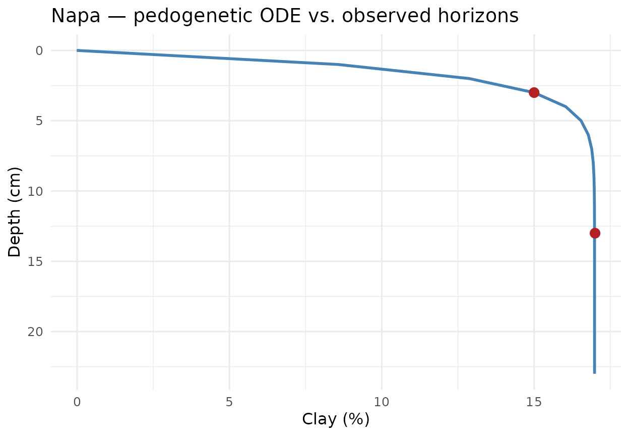

4. Multi-pedon diagnostics

Fitting the full sp4 dataset recovers an interpretable table where every row has a direct pedological meaning.

fits <- piml_profile_fit_group(
  sp4, id = "id", depth = "depth", value = "clay"
)
tab <- do.call(rbind, lapply(names(fits), function(k) {
  p <- fits[[k]]$params
  data.frame(
    pedon   = k,
    lambda0 = signif(p$lambda0, 3),
    mu      = signif(p$mu,      3),
    y_inf   = signif(p$y_inf,   3),
    y0      = signif(p$y0,      3),
    rmse    = signif(fits[[k]]$rmse, 3)
  )
}))
tab
#>                       pedon  lambda0      mu  y_inf      y0   rmse
#> log_lambda0          colusa 5.29e-03 -0.0964 61.900 22.8000 1.7600
#> log_lambda01          glenn 2.62e-01 -0.0541 34.000 -0.0232 0.0239
#> log_lambda02          kings 5.91e-02 -0.1090 27.000 -0.3850 0.0155
#> log_lambda03       mariposa 1.15e-06  2.0900 10.000 30.2000 3.1100
#> log_lambda04      mendocino 5.18e-01  0.0943 23.100  6.4900 0.0281
#> log_lambda05           napa 6.96e-01 -0.0185 17.000 -0.0119 0.0121
#> log_lambda06     san benito 3.81e-02 -0.7500 19.000  0.6070 0.0135
#> log_lambda07         shasta 3.21e-02  1.8600  0.247 14.2000 0.0103
#> log_lambda08 shasta-trinity 4.43e-02 -0.0160 75.800 18.7000 1.6100
#> log_lambda09         tehama 5.77e-03 -0.5500 32.000 23.9000 0.0290

5. Non-physical baselines

Two baselines bound the improvement claim: the mean predictor and the linear-in-depth regression. A meaningful PIML gain should come from the physical constraint, not from extra parameters.

baseline_rmse <- function(sub, target) {
  y <- sub[[target]]
  c(mean   = sqrt(mean((y - mean(y))^2)),
    linear = sqrt(mean(stats::residuals(
                     stats::lm(y ~ sub$depth))^2)))
}
bench <- do.call(rbind, lapply(split(sp4, sp4$id), function(sub) {
  bl <- baseline_rmse(sub, "clay")
  data.frame(pedon = sub$id[1],
             piml  = fits[[sub$id[1]]]$rmse,
             mean_baseline = bl["mean"],
             linear_baseline = bl["linear"])
}))
bench
#>                         pedon       piml mean_baseline linear_baseline
#> colusa                 colusa 1.75694932     12.871966       3.0163775
#> glenn                   glenn 0.02392376      4.500000       0.0000000
#> kings                   kings 0.01548473      9.797959       2.5628166
#> mariposa             mariposa 3.11248566      3.112475       2.7467763
#> mendocino           mendocino 0.02812509      4.320494       2.5935243
#> napa                     napa 0.01209286      1.000000       0.0000000
#> san benito         san benito 0.01352761      3.500000       0.0000000
#> shasta                 shasta 0.01031422      0.000000       0.0000000
#> shasta-trinity shasta-trinity 1.61442621     16.697305       3.0480840
#> tehama                 tehama 0.02900815      3.559026       0.8360796

6. Neural ODE variant

For profiles where the mono-asymptotic prior is violated — illuviated bulges, E horizons beneath A, buried paleosols — edaphos offers a Neural ODE alternative (Chen et al. 2018): $\frac{dy}{dz}=f_{\theta}(z,y),\qquad f_{\theta}=\text{MLP}(z,y;\,\theta). \tag{3}$ The forward map is a fixed-step RK4 integrator written directly in torch, so training back-propagates the squared-error loss through the whole trajectory: $$ \mathcal{J}_{\text{NODE}}(\theta) \;=\;\sum_{j}\Bigl( \underbrace{\int_{0}^{z_{j}}f_{\theta}(z,y(z))\,dz +y_{0}}_{\text{RK4 rollout}} \;-\;y_{j}\Bigr)^{2}. $$

nn_fit <- piml_neural_ode_fit(
  depths  = napa$depth, values = napa$clay,
  hidden  = c(16L, 16L), epochs = 500L,
  seed    = 1L, verbose = FALSE
)
nn_fit
pred_nn <- data.frame(depth = grid_z,
                       clay  = predict(nn_fit, grid_z))

ggplot() +
  geom_line(data = pred_napa, aes(clay, depth,
            colour = "Parametric ODE"), linewidth = 1) +
  geom_line(data = pred_nn,   aes(clay, depth,
            colour = "Neural ODE"),     linewidth = 1) +
  geom_point(data = napa, aes(clay, depth),
             size = 3, colour = "firebrick") +
  scale_y_reverse() +
  scale_colour_manual(values = c("Parametric ODE" = "steelblue",
                                  "Neural ODE"    = "darkgreen")) +
  labs(x = "Clay (%)", y = "Depth (cm)",
       colour = NULL,
       title = "Napa — parametric vs. Neural ODE") +
  theme_minimal(base_size = 12)

7. Pillar 2 × Pillar 5 — the physics gate

Given a PIML fit (parametric or neural), the helper [al_physics_gate_piml()][al_physics_gate_piml] constructs a rejection function: candidates whose predicted target falls outside the envelope $[\min(y_{0},y_{\infty}),\,\max(y_{0},y_{\infty})]$ inflated by a safety_factor are eliminated from the greedy Active-Learning selection (see the Pillar 5 vignette).

gate <- al_physics_gate_piml(fit_napa, safety_factor = 1.2)
cand_dummy <- data.frame(dummy = 1:4)
gate(cand_dummy, predicted_mean = c(10, 25, 200, -5))

A hierarchical extension ([piml_hierarchical_fit()][piml_hierarchical_fit]) jointly fits a covariate-conditioned Neural ODE across pedons, delivering a per-location envelope that [al_physics_gate_piml_hierarchical()][al_physics_gate_piml_hierarchical] feeds back into Pillar 5.

8. Bayesian posterior over the ODE parameters

[piml_profile_fit()][piml_profile_fit] returns a single point estimate. For any honest downstream use — propagating parametric uncertainty into a SOC-stock prediction, tuning a Pillar 5 Active-Learning acquisition under correct epistemic variance, reporting publishable parameter intervals — we need the posterior $p(\lambda_0, \mu, y_\infty, y_0 \mid \text{depths}, \text{values})$ , not just the MAP.

The function [piml_profile_fit_bayesian()][piml_profile_fit_bayesian] returns that posterior through two nested approximations:

Laplace approximation (default, O(ms) per pedon). Gaussian posterior whose mean is the MAP and whose covariance is the inverse observed Fisher information at the MAP (C. M. Bishop 2006, sec. 4.4). Accurate when the posterior is well-identified; every call pre-samples 2 000 draws from $N(\text{MAP}, \Sigma)$ for predictive convenience.
Adaptive random-walk Metropolis (Haario, Saksman, and Tamminen 2001) (~seconds per pedon). Proposal covariance starts at the Laplace covariance, scaled by the Roberts–Gelman–Gilks optimal factor $(2.38)^2 / d$ , and is updated online by Haario recursion after a warm-up period — so non-Gaussian or multimodal posteriors are captured faithfully where Laplace would paper over them.

library(edaphos)

depths <- c(5, 15, 30, 60, 100)
values <- c(25, 18, 12, 8, 6.5)

fit_bayes <- piml_profile_fit_bayesian(depths, values,
                                         method = "laplace", seed = 1L)
fit_bayes
#> <edaphos_piml_bayes>
#>   method     : laplace
#>   n draws    : 2000
#>   sigma (noise): 0.1653
#>   posterior summary (natural scale):
#>  parameter      mean       sd      q2.5       q50    q97.5
#>    lambda0  0.049297 0.002576  0.044338  0.049178  0.05456
#>         mu  0.004304 0.005185 -0.006121  0.004381  0.01402
#>      y_inf  6.099539 0.494554  5.152917  6.092925  7.08908
#>         y0 30.235724 0.457493 29.318151 30.236646 31.14020

predict(fit_bayes,
         newdepths         = c(10, 20, 40, 80),
         interval          = 0.95,
         include_obs_noise = TRUE,
         seed              = 1L)
#>   depth      mean        sd     lower     upper
#> 1    10 20.993046 0.2151183 20.584167 21.390906
#> 2    20 15.493301 0.2146955 15.061513 15.954735
#> 3    40 10.056425 0.2279395  9.605178 10.494935
#> 4    80  7.031722 0.2363028  6.633251  7.457589

include_obs_noise = TRUE adds Gaussian observation noise with the MAP-estimated $\sigma$ onto every predictive draw, so the returned interval represents the predictive distribution of a future observation rather than the uncertainty on the mean function alone.

For the Neural-ODE variant the variational analogue is a deep ensemble (Lakshminarayanan, Pritzel, and Blundell 2017): K independent networks trained from different random seeds produce an empirical posterior whose mean and variance approximate the Bayesian predictive posterior (Wilson and Izmailov 2020).

ens <- piml_neural_ode_fit_ensemble(depths, values,
                                       K = 5L, epochs = 300L, seed = 1L)
predict(ens, newdepths = c(10, 20, 40, 80), interval = 0.9)

9. Discussion and roadmap

The parametric ODE is mono-asymptotic and therefore optimal for properties that decay monotonically toward a parent-material value (SOC, some nutrients) but suboptimal for bimodal profiles, which the Neural ODE handles by construction. Three complementary directions remain on the roadmap:

Mass-conservation soft constraints — augment the Neural ODE loss with a term penalising deviations from an integrated mass balance (Minasny et al. 2017).
Adjoint-method Neural ODE — for pedons deeper than 2 m, the back-propagation graph becomes memory-bound; the adjoint method of (Chen et al. 2018) eliminates that scaling.
Hierarchical Bayesian pooling — extending [piml_hierarchical_fit()][piml_hierarchical_fit] to the posterior regime that [piml_profile_fit_bayesian()][piml_profile_fit_bayesian] already exposes for single pedons, with covariate-conditioned priors over $(\lambda_0, \mu, y_\infty, y_0)$ .

References

Bishop, C. M. 2006. Pattern Recognition and Machine Learning. Springer.

Bishop, T. F. A., A. B. McBratney, and G. M. Laslett. 1999. “Modelling Soil Attribute Depth Functions with Equal-Area Quadratic Smoothing Splines.” Geoderma 91 (1-2): 27–45. https://doi.org/10.1016/S0016-7061(99)00003-8.

Chen, R. T. Q., Y. Rubanova, J. Bettencourt, and D. K. Duvenaud. 2018. “Neural Ordinary Differential Equations.” In Advances in Neural Information Processing Systems. Vol. 31.

Falbel, D., and J. Luraschi. 2023. Torch: Tensors and Neural Networks with ’GPU’ Acceleration.

Haario, H., E. Saksman, and J. Tamminen. 2001. “An Adaptive Metropolis Algorithm.” Bernoulli 7 (2): 223–42. https://doi.org/10.2307/3318737.

Jenny, Hans. 1941. Factors of Soil Formation: A System of Quantitative Pedology. New York: McGraw-Hill.

Karniadakis, G. E., I. G. Kevrekidis, L. Lu, P. Perdikaris, S. Wang, and L. Yang. 2021. “Physics-Informed Machine Learning.” Nature Reviews Physics 3: 422–40. https://doi.org/10.1038/s42254-021-00314-5.

Lakshminarayanan, B., A. Pritzel, and C. Blundell. 2017. “Simple and Scalable Predictive Uncertainty Estimation Using Deep Ensembles.” In Advances in Neural Information Processing Systems, 30:6402–13.

Malone, B. P., A. B. McBratney, B. Minasny, and G. M. Laslett. 2009. “Mapping Continuous Depth Functions of Soil Carbon Using Equal-Area Splines.” Geoderma 154 (1-2): 138–52. https://doi.org/10.1016/j.geoderma.2009.10.007.

Minasny, B., B. P. Malone, A. B. McBratney, D. A. Angers, D. Arrouays, A. Chambers, V. Chaplot, et al. 2017. “Soil Carbon 4 Per Mille.” Geoderma 292: 59–86. https://doi.org/10.1016/j.geoderma.2017.01.002.

Minasny, B., and A. B. McBratney. 2016. “Digital Soil Mapping: A Brief History and Some Lessons Learned.” Geoderma 264: 301–11. https://doi.org/10.1016/j.geoderma.2015.07.017.

Raissi, M., P. Perdikaris, and G. E. Karniadakis. 2019. “Physics-Informed Neural Networks: A Deep Learning Framework for Solving Forward and Inverse Problems Involving Nonlinear Partial Differential Equations.” Journal of Computational Physics 378: 686–707. https://doi.org/10.1016/j.jcp.2018.10.045.

Soetaert, K., T. Petzoldt, and R. W. Setzer. 2010. Solving Differential Equations in R: Package deSolve. Vol. 33. 9. Journal of Statistical Software. https://doi.org/10.18637/jss.v033.i09.

Willard, J., X. Jia, S. Xu, M. Steinbach, and V. Kumar. 2022. “Integrating Scientific Knowledge with Machine Learning for Engineering and Environmental Systems.” ACM Computing Surveys 55 (4): 66:1–37. https://doi.org/10.1145/3514228.

Wilson, A. G., and P. Izmailov. 2020. “Bayesian Deep Learning and a Probabilistic Perspective of Generalization.” In Advances in Neural Information Processing Systems, 33:4697–4708.

Pilar 2 — Physics-Informed ML for Soil Depth Profiles

Hugo Rodrigues